Fast GPU Parallel BVH
A typical Gaussian splatting scene often contain massive amount of primitives. For example, there’re around 150k Gaussians in our example truck scene. Therefore, it’ll be intractable to ray trace such scene without BVH.
As we implement the entire ray tracer in Taichi kernel, we have to implement the BVH data structure and traversal algorithm in Taichi as well. As mentioned in Taichi documentation, runtime recursion is not allowed in Taichi. This makes it challenging to implement BVH traversal algorithm as well as GPU parallel BVH construction. We’d like to cover our effort in solving those issues in this technical blog.
BVH Data Structure
Our BVH data structure is highly inspired by the BVH data structure defined in Cardinal3D.
The BVH node is defined by the following Taichi struct on GPU:
@ti.dataclass
class BVHNode:
    bound: Bound
    left: ti.i32
    right: ti.i32
    prim_left: ti.i32
    prim_right: ti.i32
    depth: ti.i32
In Scene, the entire tree is defined by a BVHNode.field() where the BVHNode at index 0 is the root node. One major difference between our implementation and the BVH implemented in Cardinal3D is we cannot resize the BVHNode array on GPU easily. Therefore, we allocate the entire array in advance and construct the tree as deep as possible until we run out of nodes. This is why the size of our BVH is set by the length of BVH array instead of depth.
GPU BVH Traversal
Since Taichi doesn’t support runtime recursion, we need to implement our own stack for DFS BVH traversal. We defined such data structure in Taichi using ti.type.vector with a fixed array size:
vec_stack = ti.types.vector(32, ti.i32)

@ti.dataclass
class Stack:
    stack: vec_stack
    top: int

    def __init__(self) -> None:
        self.stack = vec_stack(0)
        self.top = 0

    @ti.func
    def size(self):
        return self.top

    @ti.func
    def push(self, idx):
        self.stack[self.top] = idx
        self.top += 1

    @ti.func
    def pop(self):
        val = self.stack[self.top - 1]
        self.top -= 1
        return val
For each BVH node hit, we push the far child to the stack first. Then we push the close child to the stack. For each ray-scene intersection, we keep popping the stack until the stack is empty. We also implement the far child pruning mechanism by skipping ray-node intersection further than the current closest hit.
GPU Parallel BVH Construction
Theoretically, we can construct the BVH on CPU and then send the data to GPU for rendering. However, as we mentioned previously, Gaussian splatting scenes often contains large amount of primitives. This makes it extremely slow to build it on CPU. Moreover, BVH construction algorithm often traverse primitives multiple times to find optimal splits. To solve these problems, we came up with the idea of construct BVH with GPU parallelism.
BVH Build Pipeline
We start by designing a pipeline to build the BVH. Our pipeline largely follows the BVH construction algorithm we implemented in Cardinal3D:
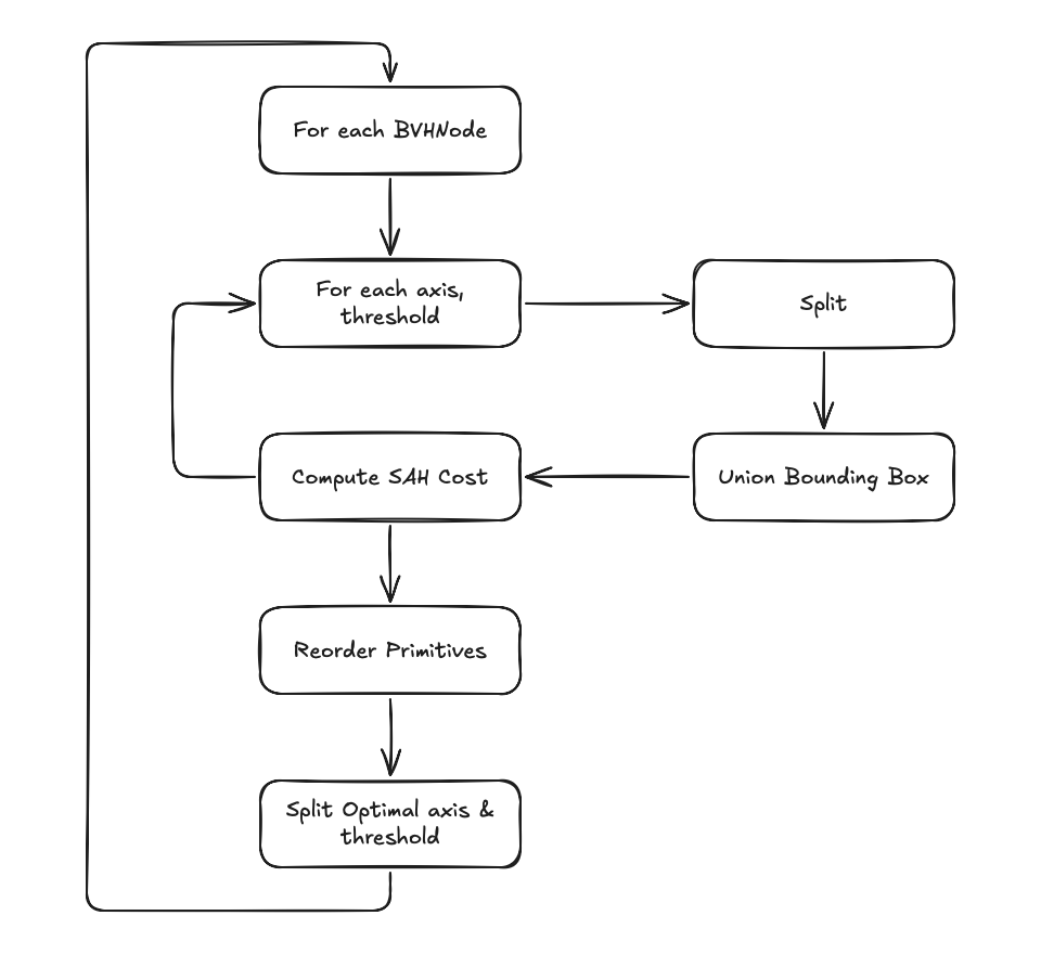
We observed hot spots in primitive split, bounding box union, and primitive reordering subroutine as they are executed over all the Gaussians for each BVHNode. Therefore, we tried to port these functions to Taichi.
Parallel Bounding Box Union, Split, and Reorder
The split kernel is defined by:
@ti.kernel
def split(start: int, end: int, axis: int, threshold: float) -> Tuple[int, int]:
    num_left = 0
    num_right = 0

    for i in range(start, end):
        gaussian = self.gaussian_field[i]
        center = gaussian.position[axis]

        if center <= threshold:
            idx = ti.atomic_add(num_left, 1)
            left_gaussian_idx[idx] = i
        else:
            idx = ti.atomic_add(num_right, 1)
            right_gaussian_idx[idx] = i

    return num_left, num_right
It takes the start and end index of a BVHNode and split all the primitives given an axis and a threshold. The function returns the number of nodes on the left child and right child.
One thing to notice is we need to use ti.atomic_add for the child size counter. This is because the kernel is parallelized over all the primitives. Using the counter directly can lead to racing condition. Please read Taichi atomic operation documentation for details.
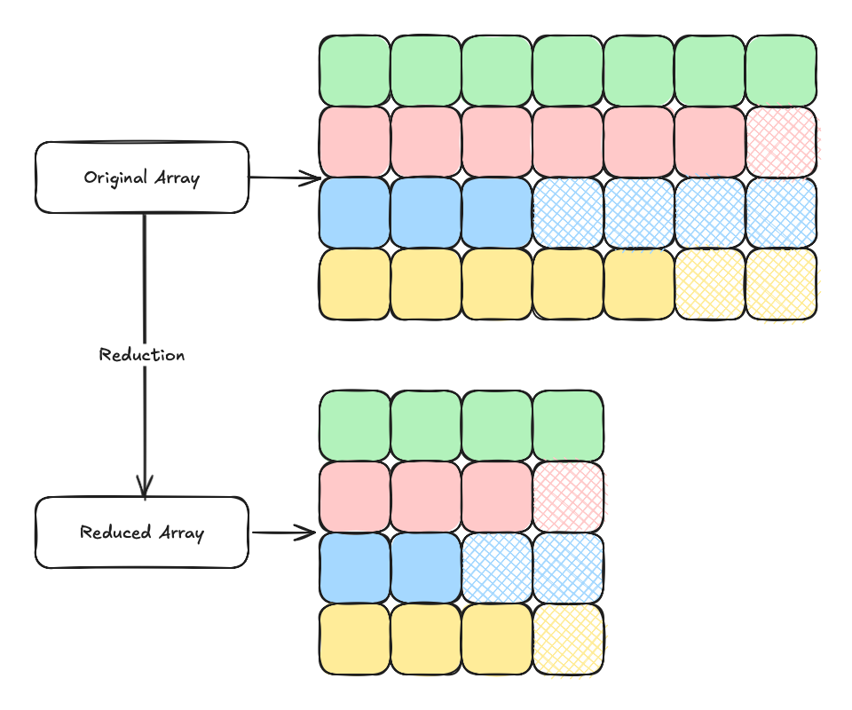
Similarly, we need to handle bounding box union with care to avoid racing condition. To solve this problem, we implemented a reduction kernel to union bounding box by pairs and the kernel is executed until the size is reduced to 1.
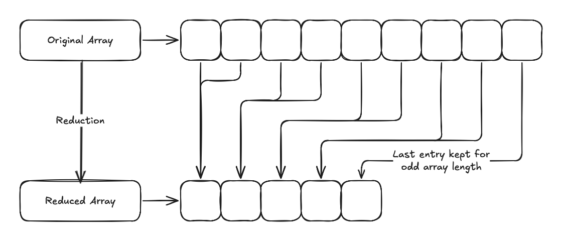
@ti.kernel
def reduction(size: int):
    for i in range(int(size / 2)):
        bbox_buf[i] = bbox_field[i * 2].union(bbox_field[i * 2 + 1])
    if size % 2 == 1:
        bbox_buf[int(size / 2)] = bbox_field[size - 1]
    for i in range(int((size + 1) / 2)):
        bbox_field[i] = bbox_buf[i]
This makes the bounding box union operation \(O(n log(n))\) instead of \(O(n)\). But being able to parallel on GPU is still worth the cost.
The reorder kernel is more straightforward. It just copy the gaussian to a buffer using the left and right index array and copy back afterward:
@ti.kernel
def reorder(start: int, end: int, num_left: int, num_right: int):
    for i in range(num_left):
        gaussian_buf[i] = self.gaussian_field[left_gaussian_idx[i]]
    for i in range(num_right):
        gaussian_buf[num_left +
                     i] = self.gaussian_field[right_gaussian_idx[i]]
    for i in range(num_left + num_right):
        self.gaussian_field[start + i] = gaussian_buf[i]
Faster BVH Build Algorithm with Axis-Threshold Level Parallel
With the aforementioned split-union-reorder-level parallel implemented, we are able to construct BVH at around 4 nodes per second. This takes the algorithm around 3 minutes to construct a BVH with 1024 nodes (we’ll skip many leaf nodes at the end of construction). With BVH at this size, the number of primitives in the leaf nodes are still to large for the ray tracer to render. However, it’ll take too long to construct a deep BVH (we tried to build a BVH with 32768 nodes in 30 minutes).
To further accelerate the BVH construction, we decide to implement axis-threshold level parallelism.
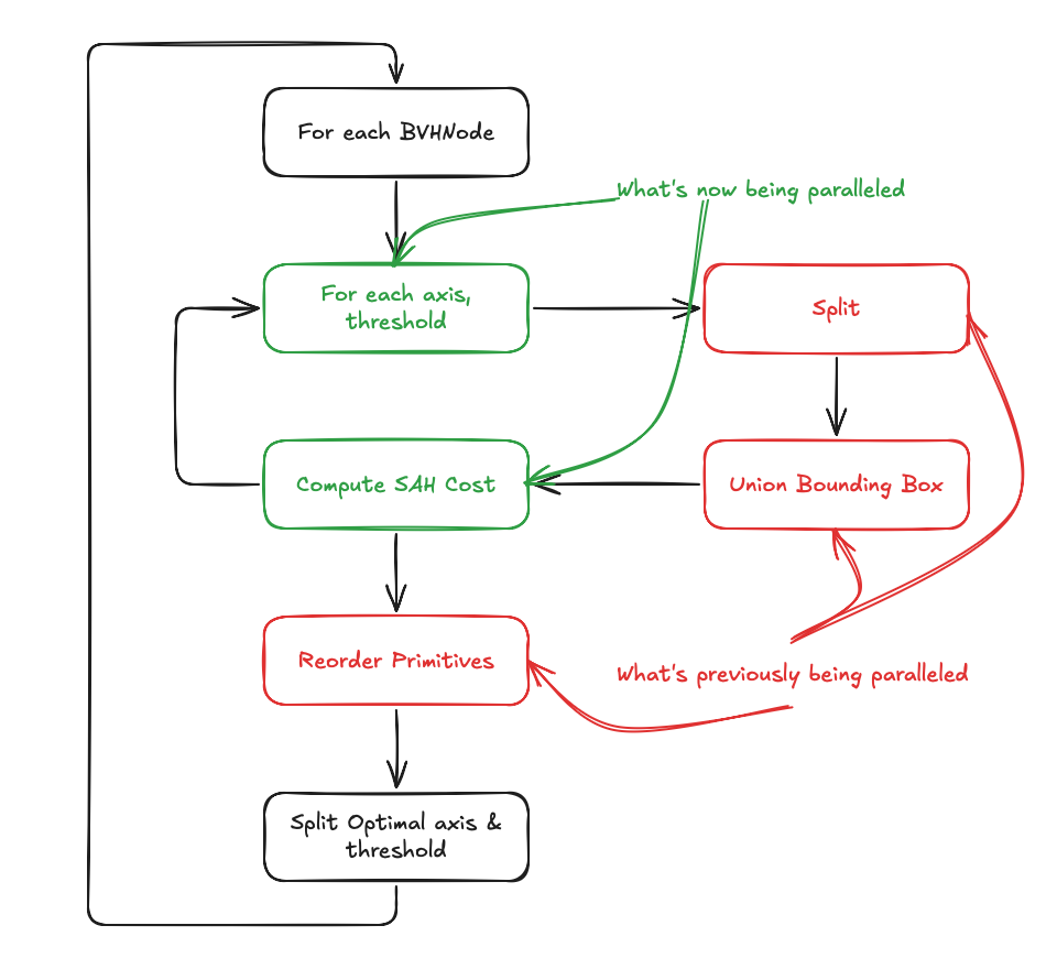
Splitting BVHNode and computing SAH can be easily parallelized to axis and threshold dimension. However, union the bounding box in parallel can be extremely challenging. This is because, for different axis and threshold, the number of primitives in each child can differ significantly. We can no longer implement a trivium reduction kernel.
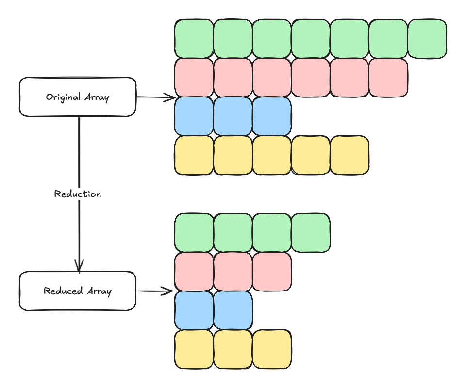
To reduce arrays of different numbers of bounding boxes in parallel, we made two key observations:
Union of two bonding boxes must contain both original bounding boxes.
Reduction of a bounding box array of size one is still itself.
With these two key observations, we can implement a reduction kernel for varying array length:
Pad all bounding box array to the same length with the last bounding box.
Reduce all arrays in parallel as the size of the longest array.
Keep track of the new size for each array independently.
Stop when the size of the longest array is reduced to one (this implies all the arrays are reduced to one).
With this implementation, we are able to construct the BVH at over 120 nodes per second. This makes it possible to construct 32k nodes in 4 minutes!