NLP and Bayesian Network
NLP (Natural Language Processing)
Bag of Word Features
Given a document $i$ and size of vocabulary $\Vert V \Vert = m$, $c_ {ij}$ is the count of word $j$ in document $i$ for $j \in [1, m]$
Bag of word feature $x_ {ij}$ is a feature correspond with document $i$, and:
\[\begin{aligned} x_ {ij} = \frac{c_ {ij}}{\sum_ {j'=1}^{m}c_ {ij'}} \end{aligned}\]N-Gram Model
The n-gram model contains 3 steps:
- Count n-gram occurrences.
- Apply laplace smoothing to the count.
- Compute the conditional probabilities.
For example, for a bigram model, the possibility of word combination $w_ 1w_ 2$ occur $P_ {{ w_ 2 \vert w_ 1 }}$ is the number of word $w_ 2$ after $w_ 1$ divided by number of word $w_ 1$ with a following word.
And the possibility of a sentence $z_ 1, z_ 2, z_ 3, \cdots, z_ d$ occur is the possibility of $z_ 1$ occur by itself times possibility of $z_ 2$ occur given $z_ 1$ and so on.
Some details of n-gram model will be given in the following article.
Unigram Model
In unigram model, the possibility of a sentence $z_ 1, z_ 2, z_ 3, \cdots, z_ d$ occur is described as following expression:
\[\mathbb{P} \{ z_ 1, z_ 2, \cdots, z_ d \} = \prod_ {t=1}^{d} \mathbb{P} \{ z_ t \}\]Here, $\mathbb{P} { z_ t }$ is the possibility of word $z_ t$ itself occur.
Mathematically, in unigram model, the occurrence of all the words are independent:
\[\mathbb{P} \{ z_ t \vert z_ 1, z_ 2, \cdots, z_ {t-1} \} = \mathbb{P} \{ z_ t \}\]For unigram model, the possibility of word $w_ t$ occur can be described as:
\[\hat{\mathbb{P}} \{ z_ t \} = \frac{c_ {z_ t}}{\sum_ {z=1}^{m} c_ z}\]Here, $c_ {z_ t}$ is the count of word $z_ t$, and $\sum_ {z=1}^{m} c_ z$ is the overall word count in the entire document.
This is called MLE (Maximum Likelihood Estimation) estimator. What the model do is maximizing the possibility of observing the sentence in the training set.
In other words, any other combination of word possibility will make the possibility of document lower.
In a MLE example, a string contains only character 0 or 1, and there are $c_ 0$ 0s and $c_ 1$ 1s. $p = \mathbb{P} { 0 }$ is the possibility 0 occurs in the document.
Thus, the possibility of the entire sentence to occur is:
\[\binom{c_ 0 + c_ 1}{c_0} p^{c_ 0} (1-p)^{c_ 1}\]To explain this expression, at one location, the possibility of 0 occur is $p$ while the possibility of 1 occur is $(1-p)$. So the possibility of a sentence with $c_ 0$ 0s and $c_ 1$ 1s to occur ignoring the combination should be $p^{c_ 0} (1-p)^{c_ 1}$. On top of that, there are $\binom{c_ 0 + c_ 1}{c_0}$ combinations for such a sentence to occur so the possibility is the one given above.
Given:
\[\binom{c_ 0 + c_ 1}{c_0} = \frac{(c_ 0 + c_ 1)!}{c_ 0!c_ 1!}\]To maximize $\binom{c_ 0 + c_ 1}{c_0} p^{c_ 0} (1-p)^{c_ 1}$, $p = \frac{c_ 0}{c_ 0 + c_ 1}$.
Bigram Model
For bigram models, the possibility of a sentence $z_ 1, z_ 2, z_ 3, \cdots, z_ d$ occur is described as following expression:
\[\mathbb{P} \{ z_ 1, z_ 2, \cdots, z_ d \} = \mathbb{P} \{ z_ 1 \} \prod_ {t=2}^{d} \mathbb{P} \{ z_ t \vert z_ {t-1} \}\]This is also called Markov property, which assume the probability of word $z_ t$ to occur only relate to word $z_ {t-1}$
Here, $\mathbb{P} { z_ t \vert z_ {t-1} }$ is the possibility of word $z_ t$ to occur given the previous word is $z_ {t-1}$.
And this possibility is calculated by:
\[\mathbb{P} \{ z_ t \vert z_ {t-1} \} = \frac{c_ {z_ {t-1}, z_ t}}{c_ {z_ {t-1}}}\]Here, $c_ {z_ {t-1}, z_ t}$ is the number of word combination $z_ {t-1}, z_ t$ occur and $c_ {z_ {t-1}}$ is the number of word $z_ {t-1}$ in the document.
Laplace Smoothing
For probability of word $z_ t$ or word combination of $z_ t \vert z_ {t-1}$:
\[\begin{aligned} \hat{\mathbb{P}} \{ z_ t \} &= \frac{c_ {z_ t}}{\sum_ {z=1}^{m} c_ z} \\ \mathbb{P} \{ z_ t \vert z_ {t-1} \} &= \frac{c_ {z_ {t-1}, z_ t}}{c_ {z_ {t-1}}} \\ \end{aligned}\]if $c_ {z_ t}$ = 0 or $c_ {z_ {t-1}} = 0$ either overfitting (predicting 0 as the possibility) or worth thing (getting x/0 => NaN) can happen.
So applying laplace smoothing lead to:
\[\begin{aligned} \hat{\mathbb{P}} \{ z_ t \} &= \frac{c_ {z_ t} + 1}{\sum_ {z=1}^{m} c_ z + m} \\ \mathbb{P} \{ z_ t \vert z_ {t-1} \} &= \frac{c_ {z_ {t-1}, z_ t} + 1}{c_ {z_ {t-1}} + m} \\ \end{aligned}\]Bayesian Network
Definition
Bayesian network is defined as a DAG (Directed Acyclic Graph) with a set of conditional probability distributions.
Each vertex represents a feature $X_ j$. Edge from $X_ j$ to $X_ {j’}$ shows that $X_ j$ directly influence $X_ {j’}$
When storing the distribution, we can only store the conditional probability given the edge information. Detail process of training and fitting will be covered in the following article.
Training
Given the DAG structure, we can find a feature $X_ j$, define $P(X_ j)$ as all parents of $X_ j$, and $p(X_ j)$ be possible values of $P(X_ j)$
Bayesian network try to find $\mathbb{P} { x_ j \vert p(X_ j) }$, which is the possibility of feature $X_ j = x_ j$ given $P(X_ j) = p(X_ j)$
To maximize this probability given the training set, we can use this expression:
\[\hat{\mathbb{P}} \{ x_j \vert p(X_ j) \} = \frac{c_ {x_ j, p(X_ j)}}{c_{p(X_ j)}}\]Here, just like n-gram model in NLP, $c_ {x_ j, p(X_ j)}$ is the count of occurrence in the training set where $X_ j = x_ j$ and $P(X_ j) = p(X_ j)$, and $c_{p(X_ j)}$ is count of occurrence where $P(X_ j) = p(X_ j)$.
Laplace Smoothing
Just like NLP, laplace smoothing can still be applied here:
\[\hat{\mathbb{P}} \{ x_j \vert p(X_ j) \} = \frac{c_ {x_ j, p(X_ j)} + 1}{c_{p(X_ j)} + \vert X_ j \vert}\]Where $\vert X_ j \vert$ is the number of possible value for feature $X_ j$
Laplace Smoothing Explanation
Laplace smoothing can be considered as a process of adding one occurrence for each possible value of $X_ j$. So the total number of occurrence should be added $\vert X_ j \vert$ times and the occurrence with specific value $x_ j$ should be added once.
Inference
To predict value using the DAG and possibility table, following expression can be used:
\[\begin{aligned} \mathbb{P} \{ x_1, x_2, \cdots, x_m \} &= \prod_ {j=1}^{m} \mathbb{P} \{ x_ j \vert x_ 1, x_ 2, \cdots, x_ {j-1}, x_ {j+1}, \cdots, x_ m \} \end{aligned}\]Here, we isolate the feature $X_ j$ and get the probability of $X_ j = x_ j$ given all other features. And since $x_ j$ is completely independent to all notes except for its parents, so:
\[\begin{aligned} \mathbb{P} \{ x_1, x_2, \cdots, x_m \} &= \prod_ {j=1}^{m} \mathbb{P} \{ x_ j \vert x_ 1, x_ 2, \cdots, x_ {j-1}, x_ {j+1}, \cdots, x_ m \} \\ &= \prod_ {j=1}^ {m} \mathbb{P} \{ x_ j \vert p(X_ j) \} \end{aligned}\]To compute the probability of $\mathbb{P} { X_ j \vert X_ {j’}, X_ {j’’}, \cdots }$, use conditional probability expression:
\[\mathbb{P} \{ X_ j \vert X_ {j'}, X_ {j''}, \cdots \} = \frac{\mathbb{P} \{ X_ j , X_ {j'}, X_ {j''}, \cdots \}}{\mathbb{P} \{ X_ {j'}, X_ {j''}, \cdots \}}\]Now we need to know the probability of $\mathbb{P} { X_ j , X_ {j’}, X_ {j’’}, \cdots }$, the tricky part is, some features may not included but they are in the dependency relationship. Here, we need to use this expression:
\[\mathbb{P} \{ X_ j , X_ {j'}, X_ {j''}, \cdots \} = \sum_ {X_ k \text{ where } k \ne j, j', j''} \mathbb{P} \{ x_ 1, x_ 2, \cdots, x_ m \}\]To explain what the f**k is going on here, we need to give two examples:
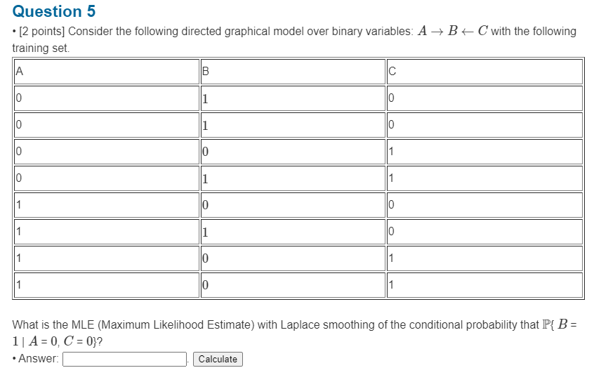
Given the bayesian network structure as $A \rightarrow B \leftarrow C$, and the training set, first train the CPT using the data:
\[\begin{aligned} \mathbb{P} \{ A \} &= \frac{4}{8} = \frac{1}{2} \implies \mathbb{P} \{ \neg A \} = \frac{1}{2} \\ \mathbb{P} \{ C \} &= \frac{4}{8} = \frac{1}{2} \implies \mathbb{P} \{ \neg C \} = \frac{1}{2} \\ \mathbb{P} \{ B \vert A, C \} &= \frac{0}{2} = 0 \implies \mathbb{P} \{ \neg B \vert A, C \} = 1 \\ \mathbb{P} \{ B \vert A, \neg C \} &= \frac{1}{2} \implies \mathbb{P} \{ \neg B \vert A, \neg C \} = \frac{1}{2} \\ \mathbb{P} \{ B \vert \neg A, C \} &= \frac{1}{2} \implies \mathbb{P} \{ \neg B \vert \neg A, C \} = \frac{1}{2} \\ \mathbb{P} \{ B \vert \neg A, \neg C \} &= \frac{2}{2} = 1 \implies \mathbb{P} \{ \neg B \vert \neg A, \neg C \} = 0 \\ \end{aligned}\]With laplace smoothing:
\[\begin{aligned} \mathbb{P} \{ A \} &= \frac{5}{10} = \frac{1}{2} \implies \mathbb{P} \{ \neg A \} = \frac{1}{2} \\ \mathbb{P} \{ C \} &= \frac{5}{10} = \frac{1}{2} \implies \mathbb{P} \{ \neg C \} = \frac{1}{2} \\ \mathbb{P} \{ B \vert A, C \} &= \frac{1}{3} \implies \mathbb{P} \{ \neg B \vert A, C \} = \frac{2}{3} \\ \mathbb{P} \{ B \vert A, \neg C \} &= \frac{2}{4} = \frac{1}{2} \implies \mathbb{P} \{ \neg B \vert A, \neg C \} = \frac{1}{2} \\ \mathbb{P} \{ B \vert \neg A, C \} &= \frac{2}{4} = \frac{1}{2} \implies \mathbb{P} \{ \neg B \vert \neg A, C \} = \frac{1}{2} \\ \mathbb{P} \{ B \vert \neg A, \neg C \} &= \frac{3}{4} \implies \mathbb{P} \{ \neg B \vert \neg A, \neg C \} = \frac{1}{4} \end{aligned}\]Note that half of the probability can be get using $\mathbb{P} { \neg x } = 1 - \mathbb{P} { x }$, so 6 probabilities are need to store in the CPT.
\[\begin{aligned} \mathbb{P} \{ B \vert \neg A, \neg C \} &= \frac{3}{4} \end{aligned}\]In another example, a bayesian network structure $A \leftarrow B \rightarrow C$ is given, and we need to find $\mathbb{P} { \neg A \vert C }$.
Here,
\[\mathbb{P} \{ \neg A \vert C \} = \frac{\mathbb{P} \{ \neg A, C \}}{\mathbb{P} \{ C \}}\]However, we cannot know $\mathbb{P} { \neg A, C }$ directly without knowing $B$, so $B$ need to be included in the calculation:
\[\begin{aligned} \mathbb{P} \{ \neg A \vert C \} &= \frac{\mathbb{P} \{ \neg A, C \}}{\mathbb{P} \{ C \}} \\ &= \frac{\mathbb{P} \{ \neg A, B, C \} + \mathbb{P} \{ \neg A, \neg B, C \}}{\mathbb{P} \{ C \}} \end{aligned}\]Here, we use $\mathbb{P} { \neg A, B, C } + \mathbb{P} { \neg A, \neg B, C }$ to include $B$. But we sum up all possible values of $B$ so that $B$ is not influencing the result anyway. This is also exactly what $\sum_ {X_ k \text{ where } k \ne j, j’, j’’} \mathbb{P} { x_ 1, x_ 2, \cdots, x_ m }$ mean in the expression above.
For $\mathbb{P} { \neg A, B, C } + \mathbb{P} { \neg A, \neg B, C }$:
\[\begin{aligned} \mathbb{P} \{ \neg A, B, C \} &= \mathbb{P} \{ \neg A \vert B \} \cdot \mathbb{P} \{ C \vert B \} \cdot \mathbb{P} \{ B \} \\ \mathbb{P} \{ \neg A, \neg B, C \} &= \mathbb{P} \{ \neg A \vert \neg B \} \cdot \mathbb{P} \{ C \vert \neg B \} \cdot \mathbb{P} \{ \neg B \} \\ \end{aligned}\]So,
\[\begin{aligned} \mathbb{P} \{ \neg A \vert C \} &= \frac{\mathbb{P} \{ \neg A, C \}}{\mathbb{P} \{ C \}} \\ &= \frac{\mathbb{P} \{ \neg A, B, C \} + \mathbb{P} \{ \neg A, \neg B, C \}}{\mathbb{P} \{ C \}} \\ &= \frac{\mathbb{P} \{ \neg A \vert B \} \cdot \mathbb{P} \{ C \vert B \} \cdot \mathbb{P} \{ B \} + \mathbb{P} \{ \neg A \vert \neg B \} \cdot \mathbb{P} \{ C \vert \neg B \} \cdot \mathbb{P} \{ \neg B \}}{\mathbb{P} \{ C \}} \end{aligned}\]