Support Vector Machine

Problems with LTU

When classify with LTU, the algorithm will stop when there’s no more error in the training set. But the result may not be the best base on the real scenario:

To solve this problem, we can introduce a thick boundary to the algorithm:

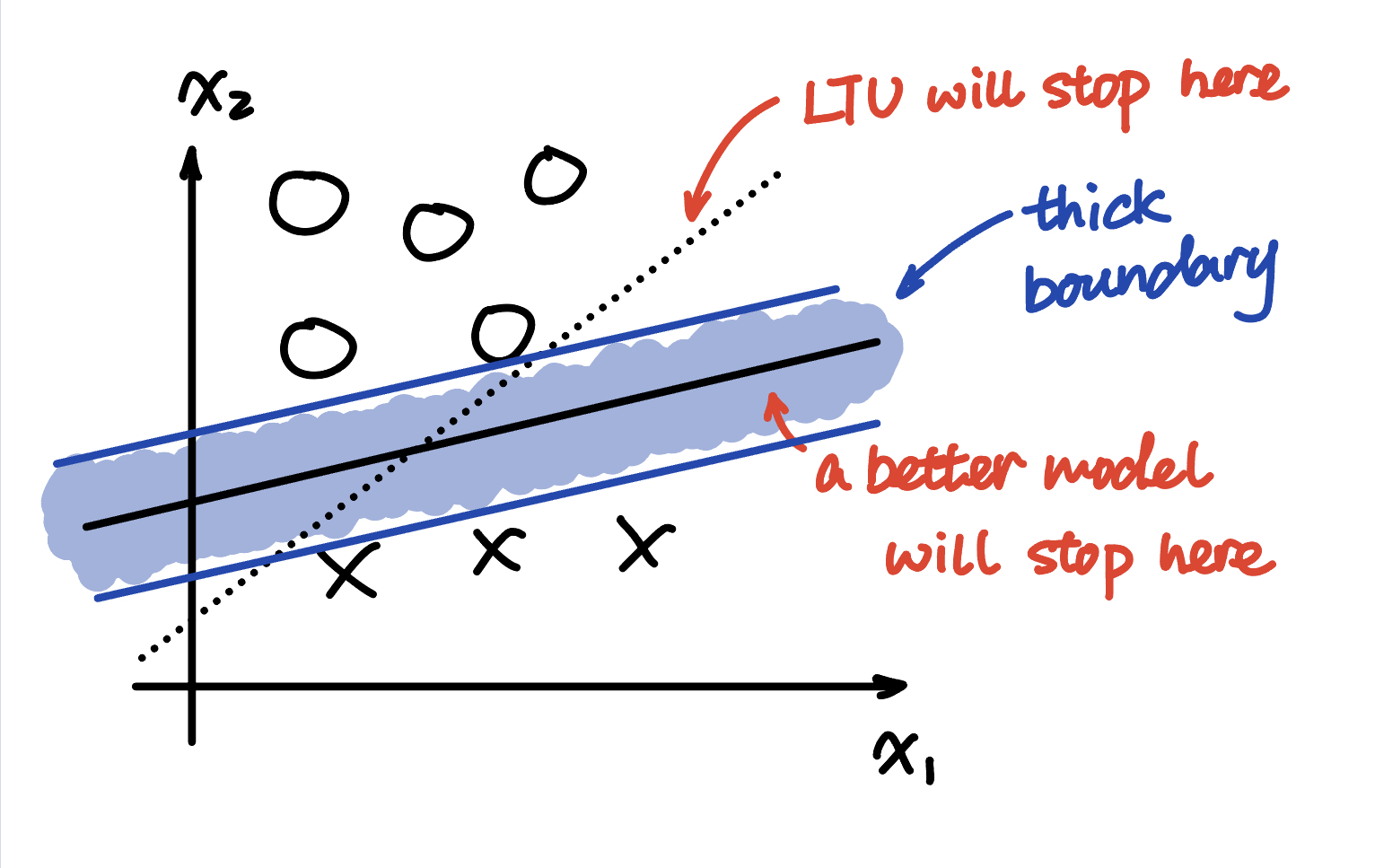
To get the best result, we need to maximize the width of the boundary. This model is called SVM (Support Vector Machine).

Support Vector Machine

Describing the Problem

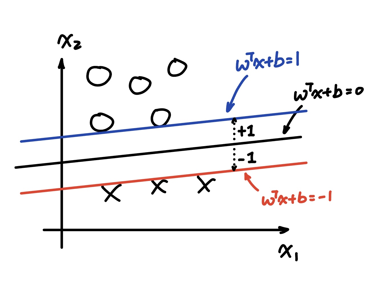
When defining the SVM, two extra planes are introduced: plus and minus plane. The plus plane (blue) is higher than $w^{T}x + b = 0$, and the minus plane (red) is lower than $w^{T}x + b = 0$.

Note that in regular LTU or logistic regression model, the plane $w^{T} + b = 0$ is just the boundary of the classification model. The real expression may be $\mathbb{1} { w^{T} + b \ge 0 }$ or $Sigmoid(w^{T} + b) \ge 0.5$.

Another thing to notice is that event if the expression seems to show that the plus plane is 1 unit away from the boundary, the real situation is the width of the boundary is not exactly 1 unit. The width of the boundary is actually determined by the weight $w$.

To prove this, we first need to realize that the normal vector of a hyperplane $w^{T}x + b = 0$ is $w$. If we normalize this normal vector we will have $w / \Vert w \Vert$, which is the unit vector of the normal vector.

The plus plane and the minus plane must be $\lambda w$ away from the boundary. So we first let vector $x_0$ be on the boundary, so that:

\[\begin{aligned} w^{T}x_0 + b = 0 \\ \end{aligned}\]

Now, $x_0 + \lambda w$ must be on the plus plane and $x_0 - \lambda w$ must be on the minus plane.

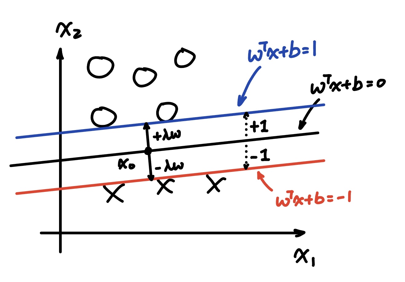
Now, solve for $w^{T}(x_0 + \lambda w) = 1$ and $w^{T}(x_0 - \lambda w) = -1$, we will have:

\[\begin{aligned} w^{T}x_0 + b &= 0 \\ x_0 &= \frac{-b}{w^{T}} \\ w^{T}(x_0 + \lambda w) &= 1 \\ w^{T}(x_0 - \lambda w) &= -1 \\ 2\lambda w^{T}w &= 2 \\ \lambda = \frac{1}{w^{T}w} \\ \end{aligned}\]

We also know that plus plane is $\lambda w$ away from the boundary, so the distance between the plus plane and the boundary is $\lambda \Vert w \Vert$. And $\Vert w \Vert = \sqrt{w^{T}w}$, so the distance between the plus plane and the boundary is:

\[\begin{aligned} \lambda \Vert w \Vert &= \lambda \sqrt{w^{T}w} \\ &= \frac{1}{w^{T}w} \sqrt{w^{T}w} \\ &= \frac{1}{\sqrt{w^{T}w}} \end{aligned}\]

The width of the boundary, which is also the distance between the plus plane and the minus plane is $\frac{2}{\sqrt{w^{T}w}}$

So the width between the plus plane and minus plane is determined by normal vector $w$. When we want to have a wider boundary, we can keep the direction of $w$ and increase the scale.

Mathematical Definition

Given the fact that the width of the boundary is $\frac{2}{\sqrt{w^{T}w}}$, we can describe the process of SVM:

\[\text{max}_w \frac{2}{\sqrt{w^{T} w}} \text{ such that } \begin{cases} (w^{T} x_i + b) \le -1, \text{if} y_i = 0 \\ (w^{T} x_i + b) \ge 1, \text{if} y_i = 1 \end{cases} \text{, given }i = 1, 2, \cdots , n\]

Note that here, $(w^{T} x_i + b) \le -1, \text{if} y_i = 0$ classifies all the points with label 0 under the minus plane and $(w^{T} x_i + b) \ge 1, \text{if} y_i = 1$ classifies all the points with label 1 above the plus plane.

On top of that, the two cases above can combined together in such form:

\[\text{max}_w \frac{2}{\sqrt{w^{T} w}} \text{ such that } (2y_i-1)(w^{T}x_i + b) \ge 1 \text{, given }i = 1, 2, \cdots , n\]

The term $(2y_i-1)$ turns into 1 when $y_i = 1$ and -1 when $y_i = 0$.

Hard SVM

When solving the weight in practice, the process of:

\[\text{max}_w \frac{2}{\sqrt{w^{T} w}} \text{ such that } (2y_i-1)(w^{T}x_i + b) \ge 1 \text{, given }i = 1, 2, \cdots , n\]

is equivalent to:

\[\text{min}_w \frac{1}{2} w^{T} w \text{ such that } (2y_i-1)(w^{T}x_i + b) \ge 1 \text{, given }i = 1, 2, \cdots , n\]

considering the fact that $\frac{2}{\sqrt{w^{T} w}}^{-1} = \frac{\sqrt{w^{T} w}}{2}$, and minimizing $\frac{w^{T} w}{2}$ will lead to a minimized $\frac{\sqrt{w^{T} w}}{2}$.

And leaving the 2 in the denominator is useful when it comes to the gradient decent.

Soft SVM

For cases that hard SVMs cannot be solved, we need to allow errors to occur. $\xi _i$ is used here in soft SVM to describe the error of i-th training point. Geometrically, $\xi _i$ is the distance between i-th point and the boundary plane. So minimizing the negative reciprocal as well as the overall error is the goal of soft SVM. This can be described as:

\[\begin{aligned} & \text{min}_w \frac{1}{2} w^{T} w + \frac{1}{\lambda} \frac{1}{n} \sum_{i=1}^{n}\xi_i \\ & \text{ such that } (2y_i-1)(w^{T}x_i + b) \ge 1 - \xi_i, \xi_i \ge 0 \\ & \text{given }i = 1, 2, \cdots , n \end{aligned}\]

In the formula above, $\frac{1}{\lambda}$ is defined as the cost of error. In cases we care about error more we can increase the cost, so that there will be less cost after training. For other cases where we care about maximizing the width of boarder, we can decrease the cost of error, so that more errors are allowed at the end of the training process.

And $\frac{1}{n}$ is used in error term is because we want to measure the average error. Without this term, error cost will be larger for cases with larger training set.

To explain why the new condition becomes $(2y_i-1)(w^{T}x_i + b) \ge 1 - \xi_i$, it is helpful to notice that without error, all the data points will satisfy the condition $(2y_i-1)(w^{T}x_i + b) \ge 1$, which is what we did in hard SVM. Allowing error is allowing data points $x_{error}$ to exist such that $(2y_i-1)(w^{T}x_{error} + b) < 1$. The actual result $\hat{y}$ generated by $x_{error}$ is $(2y_i-1)(w^{T}x_{error} + b)$, and it is $\xi_{error}$ less than the required threshold 1. So the new threshold is $(2y_i-1)(w^{T}x_i + b) \ge 1 - \xi_i$.

Notice when data points $x_i$ already satisfy the original condition $(2y_i-1)(w^{T}x_i + b) \ge 1$, $\xi_i$ will be less than 0. So another condition in the soft SVM $\xi_i \ge 0$ is just making sure introducing the error $\xi_i$ will not make the model worth when there’s no more error. You can imagine without this limitation, the model will not only try to eliminate error when the model is not accurate, but also introduce more error when the model is already accurate.

Now, we can extract $\xi_i$:

\[\begin{aligned} (2y_i-1)(w^{T}x_i + b) & \ge 1 - \xi_i \\ \xi_i & \ge 1 - (2y_i-1)(w^{T}x_i + b) \\ \xi_i & \ge 0 \end{aligned}\]

Combining the two new conditions, soft SVM can be described as:

\[\begin{aligned} \text{min}_w \frac{1}{2} w^{T} w + \frac{1}{\lambda} \frac{1}{n} \sum_{i=1}^{n}{max \{ 0, 1 - (2y_i-1)(w^{T}x_i + b) \}} \end{aligned}\]

Which is also equivalent to:

\[\text{min}_w \frac{\lambda}{2} w^{T} w + \frac{1}{n} \sum_{i=1}^{n}{max \{ 0, 1 - (2y_i-1)(w^{T}x_i + b) \}}\]

Subgradient Descent

Considering $\frac{\lambda}{2} w^{T} w + \frac{1}{n} \sum_{i=1}^{n}{max { 0, 1 - (2y_i-1)(w^{T}x_i + b) }}$ as the cost function, minimizing $w$ is similar to gradient descent in logistic regression.

While the function $max { 0, 1 - (2y_i-1)(w^{T}x_i + b) }$ is not differentiable, subgradient is introduced to solve the problem.

Subgradient requires the derivative at $x_i = 0$ greater or equal to 0 and less or equal to $\frac{\partial 1 - (2y_i-1)(w^{T}x_i + b)}{\partial x_i}$

So here comes the subgradient descent process of soft SVM:

\[\begin{aligned} \frac{\partial C}{\partial w} & \ni \lambda w - \sum_{i=1}^{n}{(2y_i-1)x_i \mathbb{1}_{\{ (2y_i-1)(w^{T}x + b) < 1 \}}} \\ \frac{\partial C}{\partial b} & \ni - \sum_{i=1}^{n}{(2y_i-1) \mathbb{1}_{\{ (2y_i-1)(w^{T}x + b) < 1 \}}} \end{aligned}\]

Here, the $\mathbb{1}_{{ (2y_i-1)(w^{T}x + b) < 1 }}$ means that when $(2y_i-1)(w^{T}x + b) \ge 1$, term $(2y_i-1)x_i$ is removed from the sum.

On the other hand, when $(2y_i-1)(w^{T}x + b) < 1$, $1 - (2y_i-1)(w^{T}x_i + b) > 0$, and thus $\xi_i > 0$, which means that the error exist. In this scenario, the gradient need to descent.

Real Life Subgradient Descent Algorithm

In practice, bias term is not included in gradient descent, and the labels are -1 and 1 instead of 0 and 1.

To achieve this, new label $z_i = 2y_i - 1$ can be used, where $y_i$ is the original label 0 or 1.

And the subgradient descent algorithm can be described as:

\[\begin{aligned} w &= (1 - \lambda) w - \alpha \sum_{i=1}^{n}z_i \mathbb{1}_{\{ z_i w^{T} x_i \ge 1 \}} x_i \\ z_i &= 2y_i - 1, i = 1, 2, \cdots, n \end{aligned}\]

Here, $\lambda$ is used as regularization parameter to avoid overfitting.

And to predict a data in the testing set, simply use $\hat{y} = \mathbb{1}_{{ w^T x_i \ge 0 }}$. Here, the bias $b$ is dropped, and $\ge 0$ instead of $\ge 0.5$ is used to classify between -1 and 1.

Kernel Trick

With feature map $\varphi$, the training set ${ (x_i, y_i) \vert i = 1, 2, \cdots , n }$ can be transfer to ${ (\varphi (x_i), y_i) \vert i = 1, 2, \cdots , n }$.

Kernel Matrix

The i-th row and i’-th column of the kernel matrix is represented by:

\[K_{ii'} = \varphi(x_i)^T \varphi(x_{i'})\]

Example:

Define feature map $\varphi (x) = (x_1^2, \sqrt{2} x_1x_2, x_2^2)$, the mapped feature of instance $i$ will be $\varphi (x_i) = (x_{i1}^2, \sqrt{2} x_{i1}x_{i2}, x_{i2}^2)$

So the $K_{ii’}$ should be:

\[\begin{aligned} K_{ii'} &= \varphi(x_i)^T \varphi(x_{i'}) \\ &= (x_{i1}^2, \sqrt{2} x_{i1}x_{i2}, x_{i2}^2)^T \cdot (x_{i'1}^2, \sqrt{2} x_{i'1}x_{i'2}, x_{i'2}^2) \\ &= x_{i1}^2x_{i'1}^2 + 2x_{i1}x_{i2}x_{i'1}x_{i'2} + x_{i2}^2x_{i'2}^2 \\ &= (x_{i1}x_{i'1} + x_{i2}x_{i'2})^2 \\ &= (x_i^Tx_{i'})^2 \end{aligned}\]