Decision Tree
Definition
When training a decision tree:
- We first need to find the most informative feature.
- Then, split the training set into subsets base on the feature.
- When all the labels in a subset are the same, stop training.
Information Entropy
To find the most informative feature, we need to use information entropy.
Binary Entropy
For binary label $y_i \in { 0, 1 }$, if the probability of $y_i = 0$ is $p_0$ and probability of $y_i = 1$ is $p_1 = 1 - p_0$. The entropy of $y_i$, or $H(y)$ is:
\[\begin{aligned} H(Y) &= p_0 log_2(\frac{1}{p_0}) + p_1 log_2(\frac{1}{p_1}) \\ &= -p_0 log_2(p_0) - p_1 log_2(p_1) \end{aligned}\]Overall Information Entropy
If label $y_i \in K$ and $K = { 1, 2, \cdots , k }$. Define $p_x$ as the probability of $y_i = x$. So that the entropy of $y_i$ is:
\[\begin{aligned} H(Y) &= \sum_{y=1}^{k}p_y log_2(\frac{1}{p_y}) \\ &= -\sum_{y=1}^{k}p_y log_2(p_y) \end{aligned}\]Conditional Entropy
Let $K_X$ be set of all the possible values of feature X, $K_Y$ be set of all the possible values of label Y.
Then, define $p_x$ is the possibility of feature $X = x$, and $p_{y \vert x}$ is the possibility of label $Y = y$ when feature $X$ is already x.
Now, the conditional entropy $H(Y \vert X=x)$ is the entropy of $Y$ when $X$ is already fixed as $x$:
\[H(Y \vert X=x) = - \sum_{y}^{K_Y}{p_{y \vert x} log_2(p_{y \vert x})}\]This is basically the same as $H(Y) = -\sum_{y=1}^{k}p_y log_2(p_y)$
Given this fact, the overall conditional entropy of $Y$ and $X$, $H(Y \vert X)$ is:
\[H(Y \vert X) = \sum_{x}^{K_X}p_x H(Y|X=x)\]This step sums up all the entropy $H(Y \vert X=x)$ with possibility of feature $X=x$, $p_x$ given x is equal to all possible values in $K_X$
Example
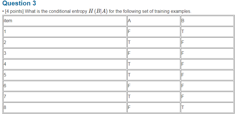
Considering $p_a$ is the possibility of feature $A = a$, and $p_{b \vert a}$ is the possibility of $B = b$ when $A = a$.
\[\begin{aligned} p_{T \vert F} &= \frac{2}{4} = \frac{1}{2} \\ p_{F \vert F} &= \frac{2}{4} = \frac{1}{2} \\ p_{T \vert T} &= \frac{0}{4} = 0 \\ p_{F \vert T} &= \frac{4}{4} = 1 \\ p_{T} &= \frac{4}{8} = \frac{1}{2} \\ p_{F} &= \frac{4}{8} = \frac{1}{2} \\ \end{aligned}\]Thus:
\[\begin{aligned} H(B \vert A=F) &= - \sum_{b}^{\{ T, F \}}{p_{b \vert F} log_2(p_{b \vert F})} \\ &= - p_{T \vert F}log_2(p_{T \vert F}) - p_{F \vert F}log_2(p_{F \vert F}) \\ &= 0.5 + 0.5 = 1 \\ H(B \vert A=T) &= - \sum_{b}^{\{ T, F \}}{p_{b \vert T} log_2(p_{b \vert T})} \\ &= - p_{T \vert T}log_2(p_{T \vert T}) - p_{F \vert T}log_2(p_{F \vert T}) \\ &= 0 \end{aligned}\] \[\begin{aligned} H(B \vert A) &= \sum_{a}^{\{ T, F \}}p_a H(B|A=a) \\ &= p_{T} H(B \vert A=T) + p_{F} H(B \vert A=F) \\ &= \frac{1}{2} \cdot 0 + \frac{1}{2} \cdot 1 \\ &= 0.5 \end{aligned}\]Information Gain
The information gain is defined as the difference between entropy and conditional entropy:
\[I(Y \vert X) = H(Y) - H(Y \vert X)\]To explain this expression, remember $H(Y)$ is the entropy of $Y$ when we do not have the information of $X$. And $H(Y \vert X)$ is the entropy of $Y$ after having information of $X$. So $I(Y \vert X)$ is the information gain of $Y$ after having the information of $X$.
Giving this explanation, it is clear that the larger information gain with respect to a particular feature $X$, the more informative that feature $X$ is.
Splitting Discrete Features
The process of finding the most informative feature $X_j$ and splitting the training set can be described as:
\[argmax_j I(Y \vert X_j)\]And after finding the feature $X_j$, split the training set into $\vert K_{X_j} \vert$ subsets. Each subset is corresponding to one feature value in $K_{X_j}$.
Here, $K_{X_j}$ is the set of all the possible values for feature $X_j$. For example, if a feature $x_{12} \in { 1, 2, 3, 5, 6 }$, the entire training set should be split into 5 subsets and each subset is correspond to one feature value in set ${ 1, 2, 3, 5, 6 }$.
Splitting Continuous Features
With discrete features, we can split a feature into multiple classes, but with continuous features it can be difficult.
One way to do that is always perform binary split on the chosen feature. And the threshold is found by trying to split on all the available instance. When finding the one with largest information gain, perform the split.
According to the expression of information gain:
\[I(Y \vert X) = H(Y) - H(Y \vert X)\]Here, Y is the label and X is the most informative feature with largest information gain.
Example
For example, when feature $x_j$ is found the most informative feature currently, list feature $x_j$ and label $y$ for all the training data:
| instance | $x_j$ | $y$ |
|---|---|---|
| 1 | 1 | 0 |
| 2 | 2 | 0 |
| 3 | 3 | 1 |
| 4 | 2 | 1 |
| 5 | 4 | 0 |
And in an example, we can find the information gain of splitting with condition $x_j < 2$, we can list that condition based on $\mathbb{1}_{{ x_j < 2 }}$
| instance | $x_j$ | $\mathbb{1}_{{ x_j < 2 }}$ | $y$ |
|---|---|---|---|
| 1 | 1 | 1 | 0 |
| 2 | 2 | 0 | 0 |
| 3 | 3 | 0 | 1 |
| 4 | 2 | 0 | 1 |
| 5 | 4 | 0 | 0 |
Thus:
\[\begin{aligned} H(Y) = \sum_{y}^{\{0, 1\}}p_{\{Y = y\}} log_2(\frac{1}{p_y}) \\ \end{aligned}\]Where:
\[\begin{aligned} p_{\{Y = 0\}} &= \frac{3}{5} \\ p_{\{Y = 1\}} &= \frac{2}{5} \\ \end{aligned}\]So:
\[\begin{aligned} H(Y) &= \sum_{y}^{\{0, 1\}}p_{\{Y = y\}} log_2(\frac{1}{p_y}) \\ &= -\frac{3}{5}log_2(\frac{3}{5}) - \frac{2}{5}log_2(\frac{2}{5}) \end{aligned}\]And:
\[\begin{aligned} H(Y \vert X_j) &= \sum_{x}^{\{ 0, 1 \}}p_{\{ X_j = x \}} H(Y \vert X_j=x) \\ \end{aligned}\]Where:
\[\begin{aligned} H(Y \vert X_j = x) &= - \sum_{y}^{\{0, 1\}}{p_{\{Y=y\} \vert \{X_j=x\}} log_2(p_{\{Y=y\} \vert \{X_j=x\}})} \end{aligned}\]Here, $X_ j$ is just an alias for $\mathbb{1}_ {{ x_ j < 2 }}$. So the probability of $p_ {{ X_ j = x }}$ is actually $p_ {{ \mathbb{1}_ {{ x_ j < 2 }} = x }}$
\[\begin{aligned} p_{\{X_j=0\}} &= \frac{4}{5} \\ p_{\{X_j=1\}} &= \frac{1}{5} \\ p_{\{Y=0\} \vert \{X_j=0\}} &= \frac{1}{2} \\ p_{\{Y=1\} \vert \{X_j=0\}} &= \frac{1}{2} \\ p_{\{Y=0\} \vert \{X_j=1\}} &= 1 \\ p_{\{Y=1\} \vert \{X_j=1\}} &= 0 \\ \end{aligned}\]So,
\[\begin{aligned} H(Y \vert X_j = 0) &= - \sum_{y}^{\{0, 1\}}{p_{\{Y=y\} \vert \{X_j=0\}} log_2(p_{\{Y=y\} \vert \{X_j=0\}})} \\ &= - \frac{1}{2}log_2(\frac{1}{2}) - \frac{1}{2}log_2(\frac{1}{2}) \\ &= -1 \\ H(Y \vert X_j = 1) &= - \sum_{y}^{\{0, 1\}}{p_{\{Y=y\} \vert \{X_j=1\}} log_2(p_{\{Y=y\} \vert \{X_j=1\}})} \\ &= - 1log_2(1) - 0log_2(0) \\ &= 0 \end{aligned}\] \[\begin{aligned} H(Y \vert X_j) &= \sum_{x}^{\{ 0, 1 \}}p_{\{ X_j = x \}} H(Y \vert X_j=x) \\ &= - \frac{4}{5} \end{aligned}\]Choice of Threshold
To make the algorithm simpler, the process above of finding threshold $x_j < x_{threshold}$ can be run for all $x_{threshold}$ in the training set instances. But a more efficient way is sort the training set based on feature $x_j$ and traversing all the discontinuous label value as possible threshold.