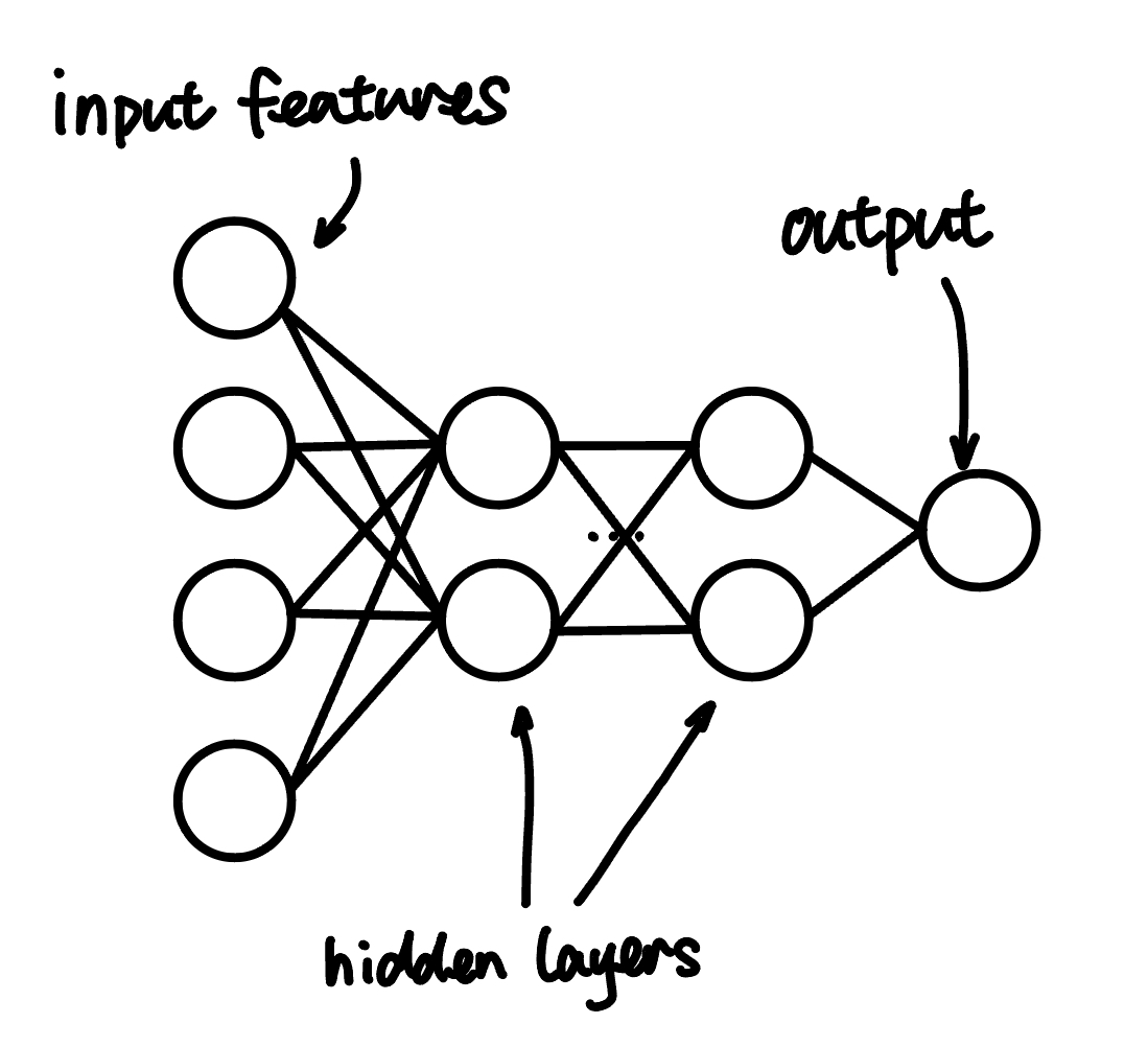
Neural Network
Basic Concepts
In logistic regression, using linear function $f$ with activation function $g$ can be described as:
\[a_i = g(w^T x_i + b)\]Although the activation function $g$ is not linear, the classification boundary determined by $f$ is still linear.
To solve this problem, logistic regressions can be stack together to form a neural network.
Each layer in the neural network takes the input from the previous layer and produces an output using logistic regression:
Mathematical Representation
For each hidden units, results from previous layers are used as input vectors.
So the representation can be described as:
\[\begin{aligned} a &= g(w^T x + b) \\ a' &= g(w^T a + b) \\ a'' &= g(w^T a' + b) \\ \hat{y} &= \mathbb{1} \{ a'' > 0 \} \\ \end{aligned}\]Gradient Descent
Since the activation function now is stacked up, the loss function which depend on the activation function is more complicated.
This lead to two problems:
- The loss function is no longer convex, so there is no longer guaranteed a global minimum.
- Chain rule need to be used to derive the loss function.
For 1, we can generate multiple random weights at the beginning of the training process. In this way, it is more likely for the algorithm to find a global minimum.
For 2, the chain rule we apply to derive the loss function is called backpropagation.
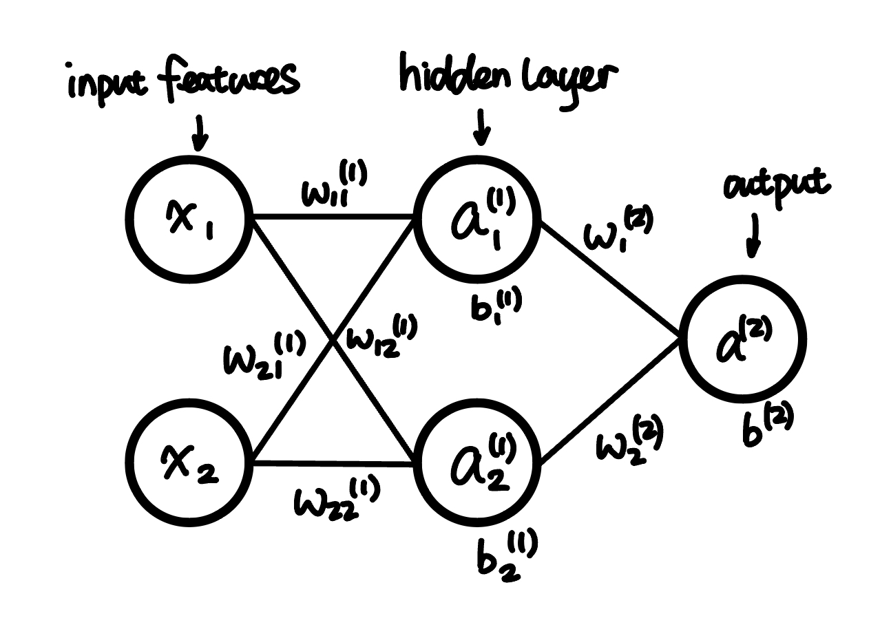
Example
This is a 2 layer neural network with 2 input features and 2 hidden units in the hidden layer:
Activation Function
For hidden unit $a_1^{(1)}$, the output is the matrix multiplication of input layer with weights $w_1^{(1)}$, which is $w_1^{(1)} = [w_{11}^{(1)}, w_{21}^{(1)}]^{T}$:
\[\begin{aligned} a_1^{(1)} &= g(w_{11}^{(1)} x_1 + w_{21}^{(1)} x_2 + b_{1}^{(1)}) \\ &= g(w_{1}^{(1)} x + b_{1}^{(1)}) \\ \end{aligned}\]The same process is applied to the hidden unit $a_2^{(1)}$:
\[\begin{aligned} a_2^{(1)} &= g(w_{12}^{(1)} x_1 + w_{22}^{(1)} x_2 + b_{2}^{(1)}) \\ &= g(w_{2}^{(1)} x + b_{2}^{(1)}) \\ \end{aligned}\]For out put unit $a^{(2)}$, the output is the matrix multiplication of hidden layer with weights $w^{(2)}$, which is $w^{(2)} = [w_{1}^{(2)}, w_{2}^{(2)}]^{T}$:
\[\begin{aligned} a^{(2)} &= g(w_{1}^{(2)} a_1^{(1)} + w_{2}^{(2)} a_2^{(1)} + b^{(2)}) \\ &= g(w^{(2)} a^{(1)} + b^{(2)}) \\ \end{aligned}\]For the loss function, we use the square error function:
\[C = \frac{1}{2} \sum_{i=1}^{N} \left( y_i - a^{(2)}_i \right)^2\]For the activation function, we use the sigmoid function:
\[g(z) = \frac{1}{1 + e^{-z}}\]Backpropagation
Finding the Gradient for $w^{(2)}$
When doing the gradient descent, we need to derive the loss function, and chain rule is still useful here.
So we first take the direction of the $C$ with respect to the activation result $a^{(2)}$:
\[\begin{aligned} \frac{\partial C}{\partial a^{(2)}} &= \frac{1}{2} \cdot 2 \cdot (y_i - a^{(2)}) \cdot (-1) \\ &= (a^{(2)} - y_i) \end{aligned}\]Remember for the sigmoid function, the derivative is:
\[g'(z) = g(z) \left( 1 - g(z) \right)\]Now, if we want to find the gradient for the weights $w^{(2)}$, we derive $a^{(2)}$ with respect to the weights $w^{(2)}$:
\[\begin{aligned} \frac{\partial a^{(2)}}{\partial w^{(2)}} &= g(w^{(2)} a^{(1)} + b^{(2)}) \cdot (1- g(w^{(2)} a^{(1)} + b^{(2)})) \cdot a^{(1)} \\ \end{aligned}\]Combing with the derivative of $C$ with respect to $a^{(2)}$, we can finally find the derivative of $C$ with respect to $w^{(2)}$:
\[\begin{aligned} \frac{\partial C}{\partial w^{(2)}} &= (a_i^{(2)} - y_i) \cdot g(w^{(2)} a^{(1)} + b^{(2)}) \cdot (1- g(w^{(2)} a^{(1)} + b^{(2)})) \cdot a^{(1)} \\ \end{aligned}\]Here the $w^{(2)}$ is just the current weight, $b^{(2)}$ is the bias for current layer, and $a^{(1)}$ is the output of the previous layer.
Note that $a^{(1)}$ is a vector with size of the number of hidden units in the first layer, so the result of above equation is also a vector with size of the number of hidden units in the first layer. And the result of $g(w^{(2)} a^{(1)} + b^{(2)}) \cdot (1- g(w^{(2)} a^{(1)} + b^{(2)}))$ is just a scalar.
The above gradient gives us the direction of the $C$ with respect to the weights $w^{(2)}$. Thus, we can update the weights $w^{(2)}$ with this gradient and learning rate.
Finding the Gradient for $w_{1}^{(1)}$ ($w_{2}^{(1)}$)
Next, we need to try to find the gradient for $w_1^{(1)}$.
To do this, we need to derive $C$ with respect to the weights $w_1^{(1)}$.
During the above calculation, we found the derivative of $C$ with respect to $a^{(2)}$:
\[\begin{aligned} \frac{\partial C}{\partial a^{(2)}} &= \frac{1}{2} \cdot 2 \cdot (y_i - a^{(2)}) \cdot (-1) \\ &= (a^{(2)} - y_i) \end{aligned}\]And given the fact that $a^{(2)} = g(w^{(2)} a^{(1)} + b^{(2)})$, we find the derivative of $a^{(2)}$ with respect to $w^{(2)}$ just now. We can do similar calculation to find the derivative of $a^{(2)}$ with respect to $a^{(1)}$:
\[\begin{aligned} \frac{\partial a^{(2)}}{\partial a^{(1)}} &= g(w^{(2)} a^{(1)} + b^{(2)}) \cdot (1- g(w^{(2)} a^{(1)} + b^{(2)})) \cdot w^{(2)} \\ \end{aligned}\]A tricky part of this calculation is that $a^{(1)}$ here is a vector with size of the number of hidden units in the first layer, and $w^{(2)}$ is also a vector with size of the number of hidden units in the first layer. Since we are trying to find the gradient for $w_1^{(1)}$, we can take only part of the result of the above equation:
\[\begin{aligned} \frac{\partial a^{(2)}}{\partial a_1^{(1)}} &= g(w^{(2)} a^{(1)} + b^{(2)}) \cdot (1- g(w^{(2)} a^{(1)} + b^{(2)})) \cdot w_1^{(2)} \\ \end{aligned}\]Now, we have the gradient for $a_1^{(1)}$. And you can see that $w_1^{(1)}$ is just the weight from $a_1^{(1)}$ to $a^{(2)}$.
Next, we need to find the gradient for $w_1^{(1)}$ with respect to the weights $a_1^{(1)}$.
Note that $a_1^{(1)} = g(w_{1}^{(1)} x + b_{1}^{(1)})$, so the gradient is:
\[\begin{aligned} \frac{\partial a_1^{(1)}}{\partial w_{1}^{(1)}} &= g(w_{1}^{(1)} x + b_{1}^{(1)}) \cdot (1- g(w_{1}^{(1)} x + b_{1}^{(1)})) \cdot x \\ \end{aligned}\]Here, the $w_{1}^{(1)}$ is the weight for vector $x$ to $a_1^{(1)}$, and $x$ is just the input vector. So the result is still a vector with size of the number of input features.
We now have the gradient of $C$ with respect to $w_1^{(1)}$:
\[\begin{aligned} \frac{\partial C}{\partial w_1^{(1)}} &= (a^{(2)} - y_i) \\ & \cdot g(w^{(2)} a^{(1)} + b^{(2)}) \cdot (1- g(w^{(2)} a^{(1)} + b^{(2)})) \\ & \cdot w_1^{(2)} \\ & \cdot g(w_{1}^{(1)} x + b_{1}^{(1)}) \cdot (1- g(w_{1}^{(1)} x + b_{1}^{(1)})) \\ & \cdot x \end{aligned}\]As $g(w^{(2)} a^{(1)} + b^{(2)})$ can be written as $a^{(2)}$, and $g(w_{1}^{(1)} x + b_{1}^{(1)})$ can be written as $a_1^{(1)}$, the above equation can be simplified to:
\[\begin{aligned} \frac{\partial C}{\partial w_1^{(1)}} &= (a^{(2)} - y_i) \cdot a^{(2)} \cdot (1- a^{(2)}) \cdot w_1^{(2)} \cdot a_1^{(1)} \cdot (1- a_1^{(1)}) \cdot x \end{aligned}\]Now you can see why this process is called backpropagation:
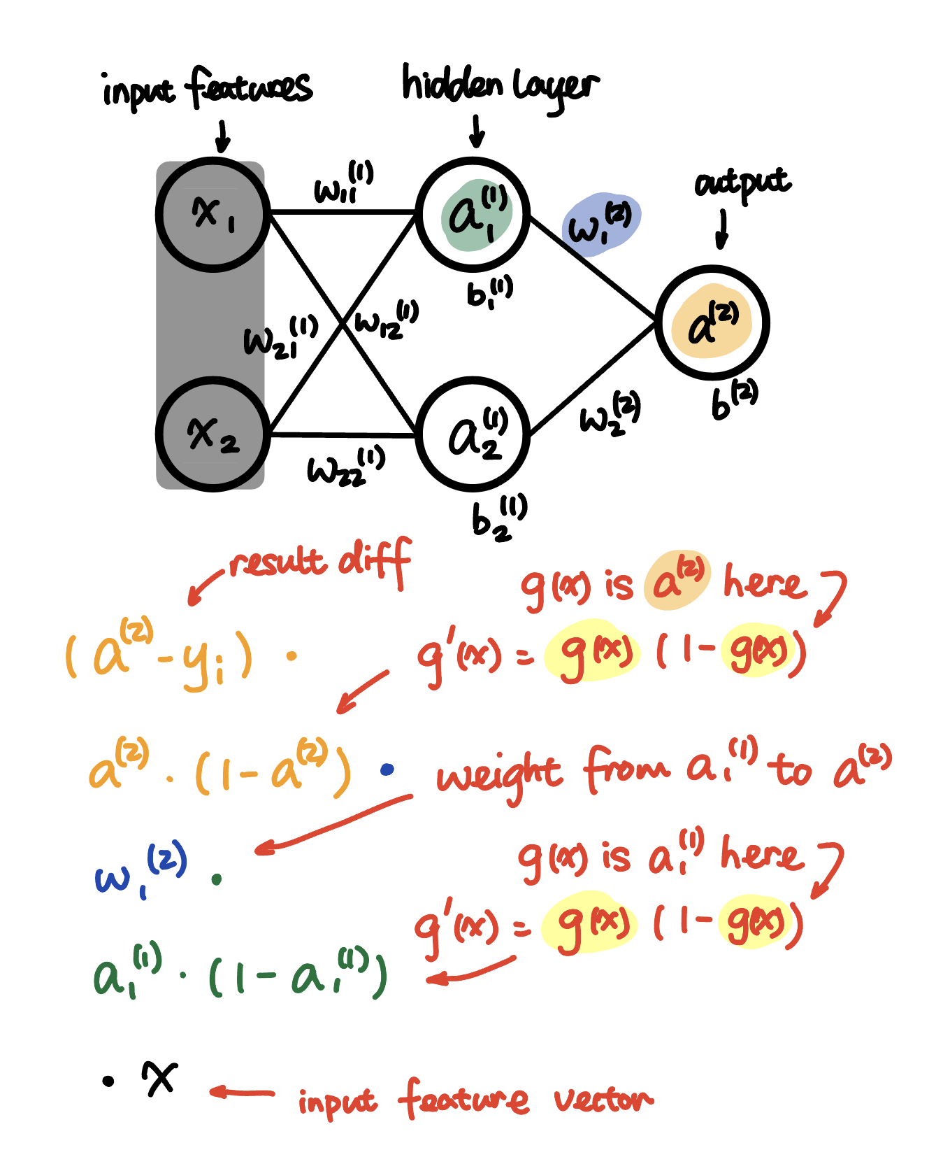
The whole process of finding the weight of a certain hidden unit starts from the final activation value output, use the value of hidden units as $g(x)$ in the $g’(x) = g(x) \cdot (1-g(x))$ and ends up with the input vector for the target hidden unit.