Notes - VoxNet - A 3D Convolutional Neural Network for real-time object recognition

Original Paper

VoxNet: A 3D Convolutional Neural Network for real-time object recognition

Introduction

This paper proposes a deep learning 3D object classification model called VoxNet. This model can convert point cloud data to voxel data and classify the object with 3D CNN.

Related Work

Point Cloud Object Recognition

Research previous to this study usually uses hand-crafted feature extractors to process point cloud data. The parameters of these feature extractors are not learnable. Therefore, much spatial information may be lost during preprocessing.

The VoxNet, in return, preserves the volumetric information. According to the authors, “it distinguishes free space from unknown space.”

2.5D CNN

Another way to process 3D data is using 2.5D convolutions, where the spatial data is stored in a depth channel. With this method, conventional CNN models can be used. However, as the method is still 2D-centric, and the depth information only comes from one viewing perspective, it may be less effective than 3D CNNs.

3D CNN

An early study and the authors’ own previous work about 3D CNN were done to leverage the volumetric representation of LiDAR data in machine learning tasks. This paper further compares several occupancy representations and proposes a model with better performance.

Approach

The main architecture of the model proposed by this paper can be divided into two parts: volumetric grid spatial occupancy representation conversion and 3D CNN classification.

Volumetric Occupancy Grid

The volumetric occupancy grid is a mathematical way to describe the state of the environment. In the grid, each voxel represents the probability of that space being occupied. The grid can be generated by several algorithms, which will be introduced later.

The authors mentioned that they chose to use this data structure for two reasons:

1. The information contained in the grid is relatively richer than other methods since each voxel can incorporate more than one LiDAR data point.
2. The data can be stored and manipulated in a relatively easy way as the data is dense.

However, the authors limited the size of the network to around $32^3$ voxels. This is probably because of the dense nature of the data structure.

Occupancy Model

Assuming there are $T$ measurements data ${ x^{t} }_{t=1}^{T}$ collected from a LiDAR sensor. Each measurement $z_{t}$ corresponds to a voxel in the space with coordinate $(i, j, k)$. $z_{t} = 1$ represents a ray hit, $z_{t} = 0$ represents a ray pass through.

There are three methods to describe the occupancy probability of a voxel mentioned in this paper.

1. Binary Occupancy Grid

The binary occupancy grid model assumes each voxel is occupied or unoccupied. Based on the data collected from the LiDAR sensor, the logged odd of a voxel $(i, j, k)$ being occupied $l_{ijk}$ will be calculated.

For a measurement $z_{t}$ on voxel $(i, j, k)$, the new logged odd $l_{ijk}^{t}$ can be calculated by:

\[l_{ijk}^{t} = l_{ijk}^{t-1} + z^{t}l_{occ} + z^{t}l_{free}\]

Where $l_{occ}$ is the logged odd of a voxel being occupied and a measurement is a hit, and $l_{free}$ is the logged odd of a voxel being occupied and a measurement is a miss.

The authors suggest that $l_{occ} = 1.38$ and $l_{free} = -1.38$. Moreover, the final log odds should be clamped to (-4, 4) to avoid numerical issues.

For the grid initialization, the probability of all the voxels being occupied is 0.5. Therefore, the logged odd $l_{ijk}^{0}$ for all $(i, j, k)$ is 0.

2. Density Grid

The density grid model assumes each voxel contains a continuous density. In this case, each voxel $(i, j, k)$ has two Beta parameters $\alpha_{ijk}^{t}$, and $\beta_{ijk}^{t}$, where $\alpha_{ijk}^{t}$ is the number of hits on the voxel and $\beta_{ijk}^{t}$ is the number of misses on the voxel.

Therefore, to update the Beta parameters of each voxel:

\[\begin{aligned} \alpha_{ijk}^{t} &= \alpha_{ijk}^{t-1} + z^{t} \\ \beta_{ijk}^{t} &= \beta_{ijk}^{t-1} + (1 - z^{t}) \end{aligned}\]

Notice that the initial values for $\alpha_{ijk}^{0}$ and $\beta_{ijk}^{0}$ are all set to 1.

The density of each voxel is finally computed by:

\[\mu_{ijk}^{t} = \frac{\alpha_{ijk}^{t}}{\alpha_{ijk}^{t} + \beta_{ijk}^{t}}\]

3. Hit Grid

The hit gird is the simplest model since it only considers hits. The hit number of each voxel is updated by:

\[h_{ijk}^{t} = min(h_{ijk}^{t-1} + z^{t}, 1)\]

Although this model is extremely simple and may discard some valuable information, the performance of this model is not significantly worse than the previous two models. Details about the comparison between different hyper-parameters will be discussed later in this note.

3D CNN Archetecture

The architecture of the model proposed in this paper is described in the following figure:

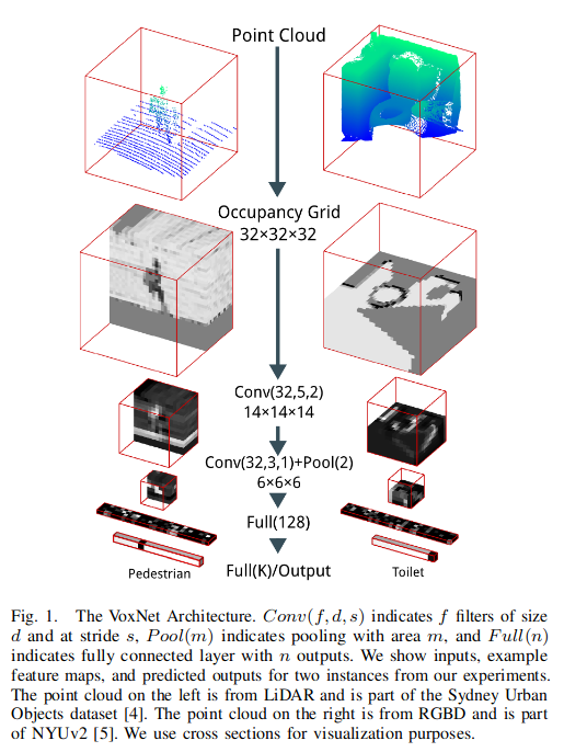
The input layer is a fixed-size grid of size $32 \times 32 \times 32$ with only one occupancy channel. Note that the occupancy should be in the range of 0 to 1. Therefore, the input is normalized to -1 to 1 by subtracting 0.5 and multiplying by 2 in the preprocessing stage. The authors mentioned that adding additional feature channels, such as RGB color channels, is possible.

Convolutional layers $C(f, d, s)$ is defined with $f$ output feature channels and $f$ learnable kernels of size $d \times d \times d \times f’$ where $d$ is the size of the kernel, and $f’$ is the number of input feature planes. The stride of the convolutional layer is defined by $s$. The authors used leaky ReLU with parameter 0.1 as the activation function for all the convolutional layers.

Pooling layers are defined by $P(m)$ where $m$ denotes the size of the pooling factor.

Fully connected layers are defined by $FC(n)$ where $n$ is the number of output neurons.

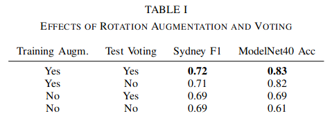
Training Data Augmentation and Voting

According to the authors, “At training time, we augment the dataset by creating n copies of each input instance, each rotated 360◦/n intervals around the z-axis. At testing time, we pool the activations of the output layer over all n copies.” Details about the augmentation and voting performance will be discussed later.

Input Resolution

As mentioned before, the spirit of the occupancy grid is to capture more detail while keeping the training and inferencing performance acceptable. The author states that “Visual inspection of the LiDAR dataset suggested a (0.2 $m^3$) resolution preserves all necessary information for the classification while allowing sufficient spatial context for most larger objects such as trucks and trees.” But the authors also admitted that “a finer resolution would help in discriminating other classes such as traffic signs and traffic lights, especially for sparser data.”

To perform object classification with higher resolution, the authors used two VoxNet at different resolutions and fused the fully connected layers to generate the final classification result. This may also be a compromise to maintain acceptable performance.

Results

The authors tested the VoxNet on multiple datasets and provided some valuable findings.

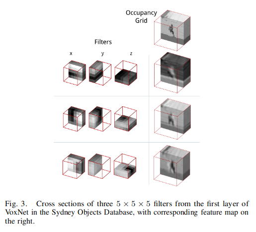
First, the authors intuitively proved that their model learned some underlying structure in the dataset by showing some intermediate layers generated by trained kernels. “The filters in this layer seem to encode primitives such as edges, corners, and ‘blobs’.”

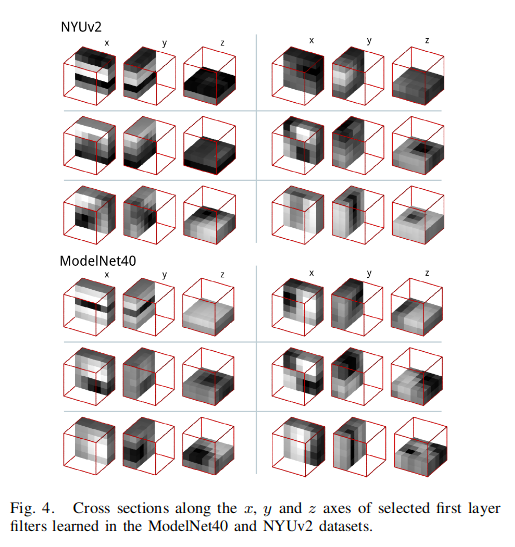
The authors also demonstrated that the kernels learned from different datasets tend to be the same, proving the effectiveness of the training design.

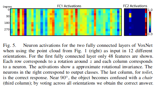
The author also showed that the model is able to learn some degree of rotational invariance by showing two fully connected layers generating similar responses to different rotations of the same input. This ability may come from the data augmentation process.

Model Evaluations

The authors first compared the model accuracy performance with different training setups. The result in the table indicates that training time augmentation is more important.

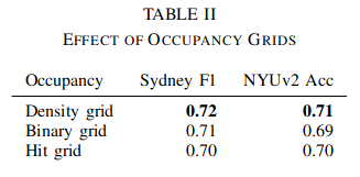
Another important finding is that VoxNet is quite robust to the different occupancy grid representations.

To show that VoxNet performs well at low input resolutions, the authors point out that the F1 score with voxels of size 0.1m and 0.2m are almost indistinguishable. Further tests on larger models are required for future research.