Notes - OctNet - Learning Deep 3D Representations at High Resolutions

Original Paper

OctNet: Learning Deep 3D Representations at High Resolutions

Introduction

This paper proposed a new CNN structure called OctNet. The goal is similar to other Sparse CNN research: reducing the memory and computational cost of CNN on sparse data. This paper specifically focuses on 3D data since the authors mentioned, “for dense 3D data, computational and memory requirements grow cubically with the resolution.”

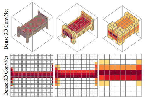
The authors also mentioned a very interesting observation in the introduction section: “We depict the maximum of the responses across all feature maps at different layers of the network. It is easy to observe that high activations occur only near the object boundaries.” This phenomenon is shown in this figure, where higher activations are indicated with darker colors:

Related Work

According to the author of this paper, traditional dense CNN only support up to 30^3 voxels. Solutions to this problem include reducing the depth of the networks. This may, in return, impact the expressiveness of the network.

Another related research is the Sparse 3D convolutional neural networks. @Anyonering discussed this paper in this discussion.

A phenomenon mentioned by the author is that the SCNN structure only supports 2x2 convolutions and therefore prevents the network from growing larger. As a result, “the maximum resolution considered in [16, 17] is 803 voxels.” Further discussion about this phenomenon will be posted here.

Octree Networks

The main contribution of this research is proposing the OctNet architecture. This model leverages the octree to store the sparse data.

However, as mentioned in the paper, “While octrees reduce the memory footprint of the 3D representation, most versions do not allow for efficient access to the underlying data.” This is mainly because it is usually difficult to access neighboring nodes in octrees. In the worst case, accessing the neighboring node may require the algorithm to traverse upward to the root node and go back to the leaf node again.

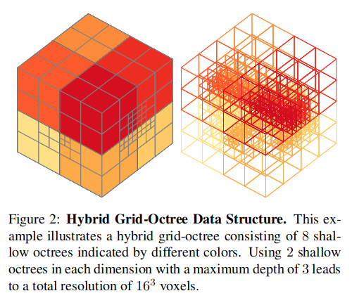
Hybrid Grid-Octree Data Structure

The authors of this paper solve the aforementioned problem by using a hybrid grid-octree data structure. Simply put, this data structure is a grid of octrees called “shallow octrees.” Shallow octrees enforce a depth constraint so that the maximum depth of the octree will be constant. When the data is large, more shallow octrees will be added to the grid, but the max depth of each octree does not change. A simpler way to understand this data structure is by considering shallow octrees as the basic building blocks of the grid.

Using shallow octrees will introduce two main benefits:

1. The algorithm does not need to traverse too many nodes to find its neighbors.
2. The fixed depth octree can be represented by a fixed length bit array. Therefore, parallel optimization can be used to accelerate the algorithm.

For example, in this figure, the structure of a shallow octree of depth three can be represented by a 73-bit array:

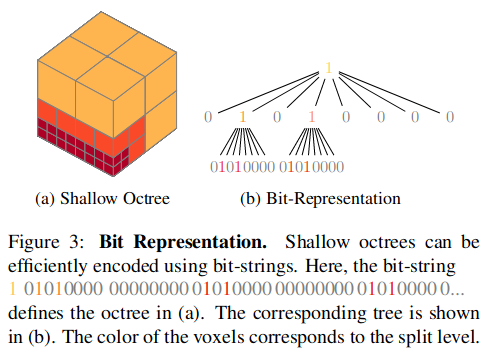
In the bit representation, 0 means there’s a data node, and 1 means there’s a split node. Note that 73 bits only covered two layers. This is because, in a shallow octree of depth 3, the third layer can only contain data nodes (represented by bit 0).

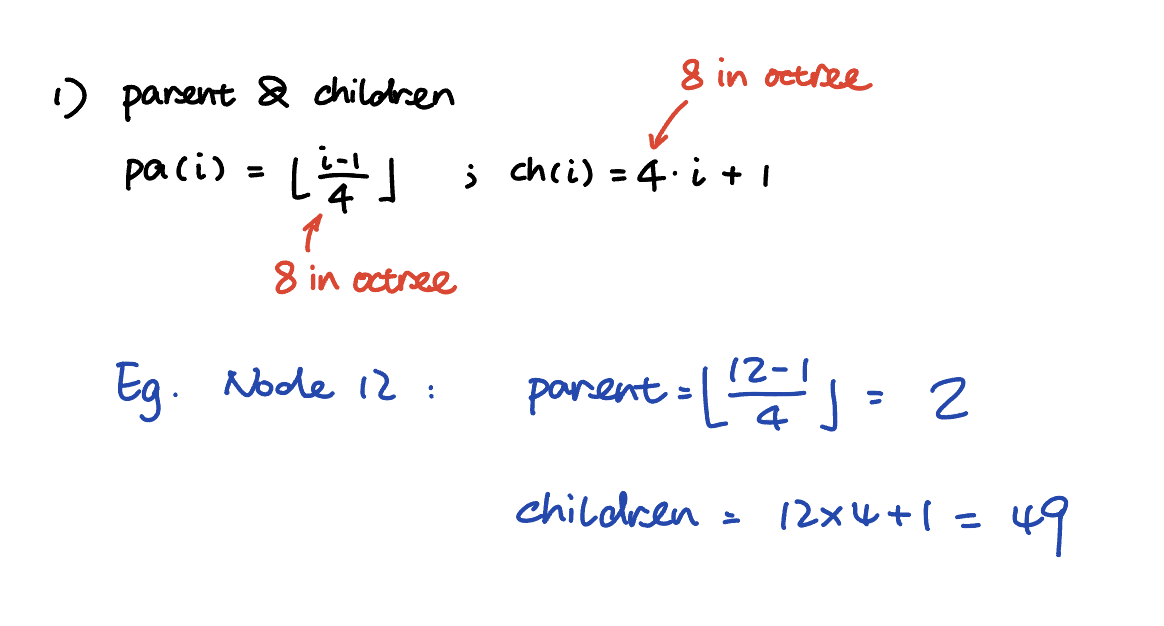
This shallow octree can store up to $8^3$ voxels, and each voxel has a corresponding bit index. The parent index and children index of a specific voxel at index $i$ can be calculated by:

\[\begin{aligned} parent(i) &= \lfloor \frac{i-1}{8} \rfloor \\ children(i) &= 8 \cdot i + 1 \end{aligned}\]

All the data (feature vectors of each data node voxel) are stored in a data container associated with the corresponding shallow octree. To access the index of the feature vector of voxel $i$ in the data container, the following expression is used:

\[dataidx(i) = 8 \sum_{j=0}^{parent(i)-1}bit(j) + 1 - \sum_{j=0}^{i-1}bit(j) + mod(i-1, 8)\]

To demonstrate how this data structure works, a simpler quadtree is used here as an example:

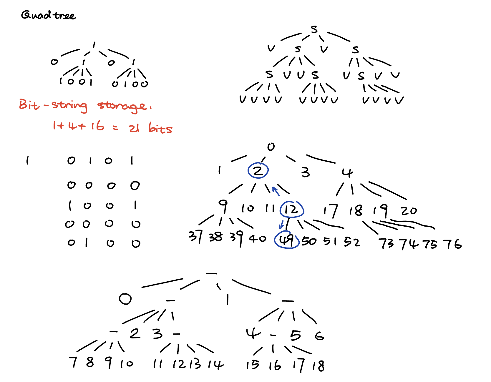
This quadtree contains six split nodes at 0, 2, 4, 9, 12, and 19.

Therefore, the bit array representation is 1 0101 0000 1001 0000 0100.

If we want to find the parent and children nodes of node 12:

The data index formula can be explained by:

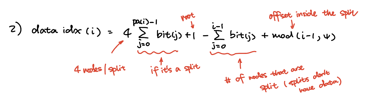
To find the data index of a certain node:

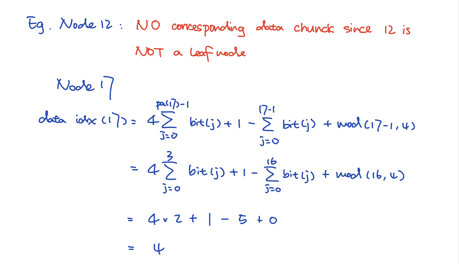
Note that the data index of a node is defined only if the node is a leaf node. Thus, finding the data index of node 12 does not make sense here, as node 12 is a split node.

Network Operations

A grid of data in a shallow octree can be represented by two forms: dense tensor $T$ and shallow octree $O$.

$T_{i, j, k}$ denotes the value of a 3D tensor T at location $(i, j, k)$, $O[i, j, k]$ “denotes the value of the smallest cell in this structure which comprises the voxel $(i, j, k)$.”

Note that an octree node may contain multiple voxels in the corresponding tensor. Therefore, multiple coordinates may point to the same data node. The authors explain this feature mathematically with “$O[i_1, j_1, k_1]$ and $O[i_2, j_2, k_2]$ with $i_1 \ne i_2 \lor j_1 \ne j_2 \lor k_1 \ne k_2$ may refer to the same voxel in the hybrid grid-octree, depending on the size of the voxels.”

Given a shallow octree structure bit array and a corresponding tensor, converting the octree to the tensor is given by:

\[T_{i, j, k} = O[i, j, k]\]

Converting the tensor to the octree can be expressed by

\[O[i, j, k] = poolvoxels_{(\bar{i}, \bar{j}, \bar{k}) \in \Omega[i, j, k]}(T_{\bar{i}, \bar{j}, \bar{k}})\]

Where $\Omega[i, j, k]$ is the set of all the voxels that are contained in the same data node as voxel $(i, j, k)$.

A naive implementation of any CNN kernel function $f$ can be done by:

\[g(O) = ten2oc(f(oc2ten(O)))\]

This implementation simply converts the octree to a tensor and converts the tensor back to an octree after applying the kernel. It’s not hard to imagine that this implementation is inefficient, and the authors do not recommend doing so.

Octree Convolution

In dense tensor, a convolution kernel $W \in \mathbb{R}^{L \times M \times N}$ can be done by

\[T_{i, j, k}^{out} = \sum_{l=0}^{L-1} \sum_{m=0}^{M-1} \sum_{n=0}^{N-1} (W_{l, m, n} \cdot T_{\hat{i}, \hat{j}, \hat{k}}^{in})\]

Where

\[\begin{aligned} \hat{i} &= i - l + \lfloor \frac{L}{2} \rfloor \\ \hat{j} &= j - m + \lfloor \frac{M}{2} \rfloor \\ \hat{k} &= k - n + \lfloor \frac{N}{2} \rfloor \end{aligned}\]

Given a shallow octree $O$, the same operation can be done with the following:

\[T_{i, j, k}^{out} = \sum_{l=0}^{L-1} \sum_{m=0}^{M-1} \sum_{n=0}^{N-1} (W_{l, m, n} \cdot O^{in}[\hat{i}, \hat{j}, \hat{k}])\]

Notice that this operation accepts an octree as the input while returning a dense tensor as the output. This is intentional, as the voxels in the same data node may be different after each convolution. However, according to the theory mentioned in the introduction part, “high activations occur only near the object boundaries.” As the octree captures these boundaries in the deep layers, it’s reasonable to convert the dense tensor back to the octree after this convolution operation.

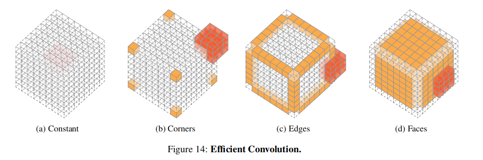
The authors also mentioned a method to compute convolutions on octrees more efficiently. Since all the voxels in an octree node contain the same feature vector, it’s possible to apply the kernel in parallel with 4 phases: constant, corners, edges, and faces. In each phase, data in some part of the kernel filter can be reused, and a relatively high cache hit rate can be achieved.

Octree Pooling

Pooling operations in octrees are done by applying $max$ or $mean$ functions on the deepest leaf nodes (eg. For a shallow octree with a max depth of 3, the average or max pooling only happens on the depth of 3 leaf nodes. This is because applying the function on other lower-depth nodes will give the same result). After pooling, the max depth of the shallow octree will decrease by 1. To solve this problem, 8 neighboring shallow octrees in the grid form a new shallow octree.

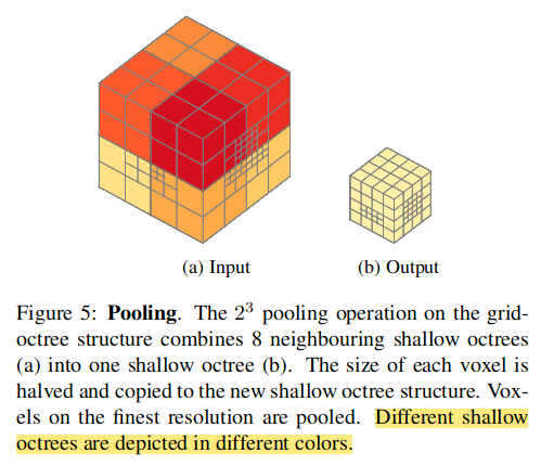
In other words, some levels of grids are pushed down to be the root of the scaled-down octrees. The broad picture of this process is: the depth of shallow octrees holds the same while the number of grids decreases.

Octree Unpooling

The unpooling process is similar to the pooling process, while the number of shallow octrees in the grid increase by a factor of 8.

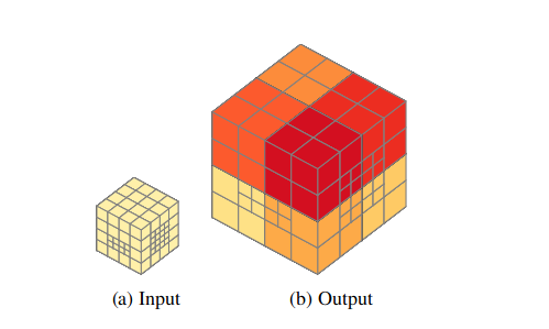
Notice that after each unpooling operation, “the tree depth is decreased.” This can be seen in the figure above: the max depth of all shallow octrees becomes 2 instead of 3. This can be problematic in some fully connected models, such as U-Net since the resolution of the hidden layer prominently decreased after the previous pooling layers.

The authors mentioned a possible solution to this problem: “To capture fine details, voxels can be split again at the finest resolution according to the original octree of the corresponding pooling layer.”

In the paper, the authors also use this method to support skip connections in the 3D semantic segmentation tasks.

A possible defect of this method is that it only supports the same sparse layout as the input for the output. This feature is acceptable when dealing with tasks such as semantic segmentation. But for high-resolution model generation or other generative tasks, the unpooling process may be suboptimal.