2023-05-14

Notes - 3D Semantic Segmentation with Submanifold Sparse Convolutional Networks

Notes: 3D Semantic Segmentation with Submanifold Sparse Convolutional Networks

Original Paper

3D Semantic Segmentation with Submanifold Sparse Convolutional Networks

Introduction

CNNs are widely used to solve many computer vision tasks, while the number of points on the grid grows exponentially with its dimensionality.

Traditional neural networks are optimized for dense data. Therefore, the negative impact on performance may manifest when sparse data are processed (3D point cloud data, for example).

To solve this problem, Submanifold Sparse Convolutional Network (SSCN) is proposed in this paper.

Previous studies about sparse convolutional networks have been done in Vote3Deep: Fast Object Detection in 3D Point Clouds Using Efficient Convolutional Neural Networks, Sparse 3D convolutional neural networks, and OctNet: Learning Deep 3D Representations at High Resolutions.

Vote3Deep achieves greater sparsity after convolution with ReLUs and a special loss function.

Sparse 3D CNN considered all the sites with at least one active input as active. This will lead to a decrease in sparsity after each convolutional layer. This behavior will be discussed later in this note.

OctNet uses oct-trees to handle sparse data, which is a common trick in computer graphics.

Spacial Sparsity for ConvNets

A d-dimensional CNN is a network that takes (d+1)-dimensional tensors as input: These tensors contain d spacial dimensions and one feature space dimension.

For example, a traditional 2D CNN accepts a 3D tensor as the input. 2 dimensions correspond to the coordinates of each pixel. While an extra dimension stores the color channels as features.

“The input corresponds to a d-dimensional grid of sites, each of which is associated with a feature vector.” Here, a site is defined as a point in the spatial dimension.

A site is active if any element in the feature vector is not in its ground state, e.g. if it is non-zero.

Note that a site corresponds to one feature vector, and this feature vector may contain multiple features. The site will be defined as active when at least one of the features is not in the ground state. The authors describe this behavior as d-dimensional activity in (d+1)-dimension tensors.

In the paper that introduced Sparse 3D CNN, a site in a hidden layer will be activated if any of the sites in the layer that it takes as input is active. In this case, the activity structure of each hidden layer can be calculated from the previous layer.

This implementation also leads to a decrease in sparsity as data propagates through the network. With 3x3 convolution layers in a d-dimensional network, a layer with $1$ active site will contribute to $(1+2n)^d$ active sites after n layers. The advantage of handling sparse data will soon be compromised after several convolution layers. And this problem is harmful in some structures, such as U-Net, as most sites may be active in low-resolution layers after convolutions and polling.

This issue is less severe when the input data is relatively dense. But the aforementioned data dilation issue is problematic in cases that incorporate d-dimensional structures in (d+1)-dimensional input (a 2d surface in 3d space). A classical example is 3D point-cloud data, which often represents 2d surfaces.

The authors refer to this problem as the “submanifold dilation problem.”

Submanifold Convolutional Network

In this paper, the authors propose a solution to the submanifold dilation problem that “restricts the output of the convolution only to the set of active input points.”

The visualization of this structure is demonstrated in Fig 2 and Fig 3:

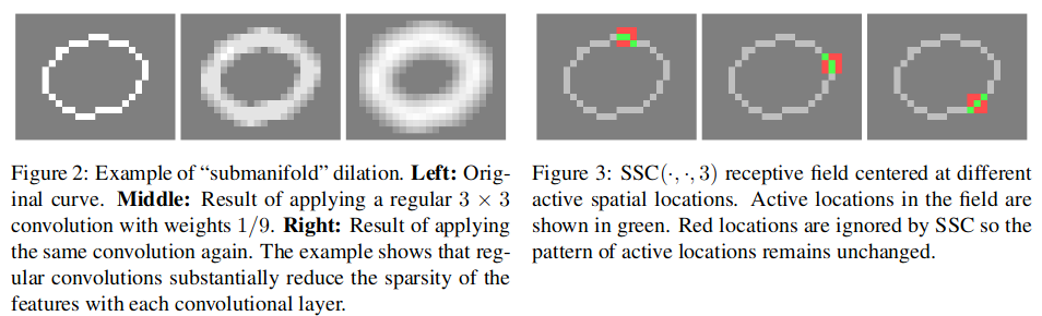
Fig 2 shows that after each convolution layer, the active sites expand, and the sparsity decrease. While in Fig 3, the sparsity of each hidden layer is preserved by forcing the active sites in all layers to remain the same.

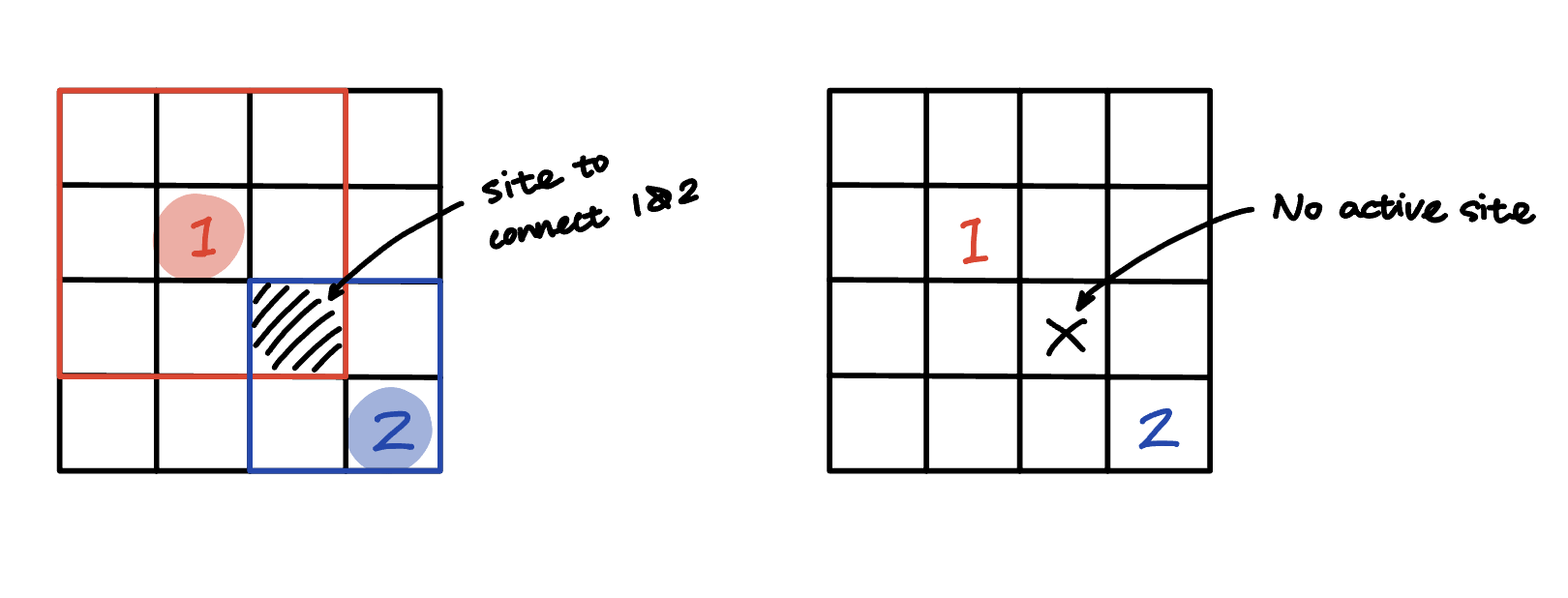
Information Flow Between Connected Components

In the paper, the author mentioned that “two neighboring connected components are treated completely independently,” and this issue can lead to loss of information in hidden layers.

Specifically, in the following example, the submanifold dilation version of SCNN can connect sites 1 and 2 with the shaded site. The constant activity implementation cannot establish this connection as the site is inactive.

Sparse Convolutional Operations

A sparse convolution $SC(m, n, f, s)$ is defined with m input feature planes, n output feature planes, a filter with size f, and stride s.

Here, “m input feature planes” means for each site, there is an m-dimensional feature vector.

A submanifold sparse convolution $SSC(m, n, f, s)$ is defined similarly to $SC$, while all the active sites are restricted to be the same as active input sites.

In the paper, $a$ is defined as the number of active inputs to the spacial location.

implementation

To store the data in each layer, a value matrix of size $a \times m$ and an indexing hash table is used. Note that these two data structures are used to store layer data, such as input data or hidden layer state. The weights of the neural network are stored in another matrix.

Given a convolution with filter size $f$, there are $f^d$ sites in the previous layer that contribute to the current site. $F = { 0, 1, \cdots , f-1 }^d$ denote the spatial size of the convolution filter.

A rule book $R = (R_{i} : i \in F)$ contains $f^d$ rule matrices that correspond to each position in the convolution filter. Detailed implementation will be explained later.

An $SC(m, n, f, s)$ with $a$ active input sites is implemented by the following steps:

The output hash table and value matrix are built by iterating all the active input sites and adding all the output sites that in the filter range of the input sites to the output hash table. The hash table maps a coordinate on the spacial dimension to a row in the value matrix. Thus, the size of the value matrix is $sizeof(hashtable) \times n$. The rule book is also built on-the-fly. For each active input $x$ located at point $i \in F$ that gives the output $y$, a row (input-hash(x), output-hash(y)) is added to the rule $R_i$
For each $i \in F$, there is a parameter matrix $W_i$ of size $m \times n$. This matrix is used to calculate the feature vector at location i. To apply a convolution kernel, loop for each row $(j, k)$ in rule $R_i$, multiply the j-th row of the input feature value matrix, and add to the output feature value matrix.

Although this implementation does not incorporate any use of VDB or even oct-tree data structure, there’s still SIMD or SIMT optimization opportunity since step 2 mentioned above can be executed in parallel.

However, the detailed performance of this operation, when compared with the oct-tree implementation, needs further benchmarks.